Idea and package-selection
For the general pipeline I decided to work in python and find a way to efficiently compute cubical persistence for my collection of Lenia lifeforms. I decided to work with the package giotto-tda, which comes with all the basic functionalities that I needed for this project and can be used directly with my .vti-files.
Cubical Persistence
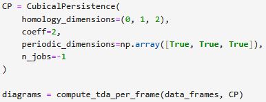
After loading in the .vti files (and reordering them to the correct shape) one can almost immediatly apply the CubicalPersistence() function provided by giotta-tda.
|
Note that periodic_dimensions are all set to True, since Lenia supports periodic boundary conditions.
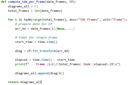
Here the Cubical Persistence computation is carried out by the function 'compute_tda_per_frame()':
|
The primary work is done by the fit_transform() function contained in giotto-tda's CubicalPeristence import. I also applied tqdm() to track the time for computation, as some lifeforms took up to 6 hours to compute, dependent on the number of frames and their resolution. For a given lifeform the results are then saved in a variable called 'diagrams'.
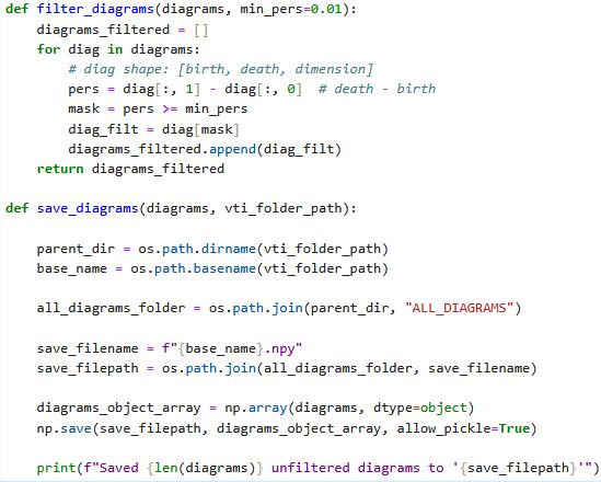
I furthermore included a functionality to save the respective diagrams after computation and to filter them according to an arbitrary minimal persistence.
|
Life-Death-Diagrams
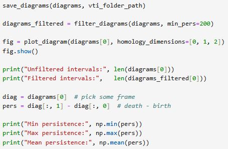
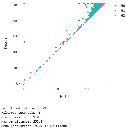
From these diagrams alone one can easily plot the persistence diagram, here given for an example lifeform.
|
In this example it is already highly visible that some lifeforms contain a large number of low persistency features. In this specific case there were 795 features detected before filtering resulted in only 8 'true' features: Showcased here is the persistence diagram before filtering, as well as some metrics computed before and during filtration. Note that we used a fairly high minimal persistence of 200 here.
|
Betti-numbers over time
One can then easily obtain the Betti-numbers for a given frame by summing over their occurances in the filtered diagram:

|
However, I am not only interested in the topology of a single frame, but particularly how it evolves over time. Therefore I am particularly interested in the change of Betti numbers over time, as well as a way to visualize it:
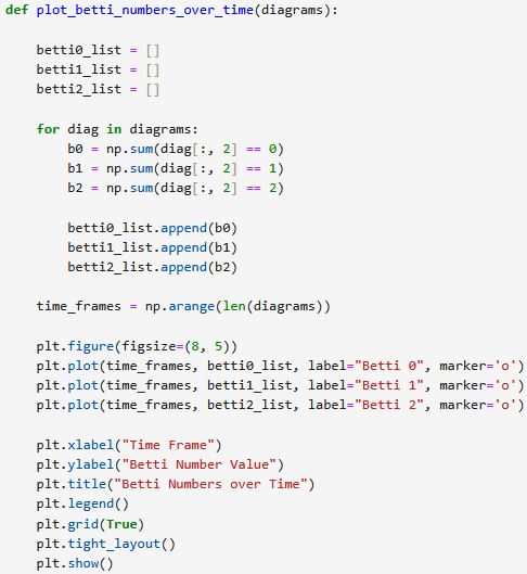
|
Which yields a fairly intuitive visualization of what is going on, as seen in this short sample set of three widely spaced frames of a single lifeform:
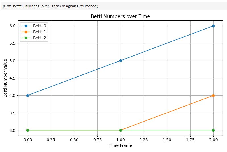
In this particular case we observe a lifeform that seems to have a constant number of three voids (which as we will see in the case study section are hollow spheres), an increasing number of disconnected components and the formation of a loop.
Automated filtration value estimate through Otsu's method
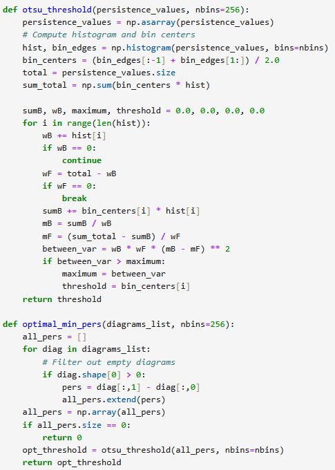
Up to this point, I was mainly playing around with the functionalities of giotto-tda. However, I found it quite bothersome to manually choose minimal persistence values for every single lifeform, as fitting values did not seem to be consistent across different lifeforms. This is why I implemented an automatic functionality to determine a good minimal persistence using Otsu's method.
The idea is to gather all persistence values from a diagram and use Otsu's algorithm to choose a fitting threshold to separate the low persistence population (probably noise) from the high persistence population (probably the true data signal) and then apply the obtained threshold as min_persistence value.
|
I furthermore included a helper function to see how the obtained threshold is distributed throughout all lifeforms:
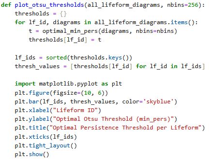
|
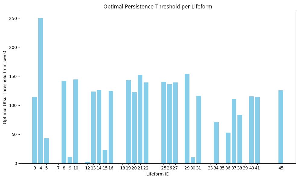
Which returns the following distribution:
Topological classification
It is noticeable that our lifeforms can already be grouped according to their ideal minimal persistence, or by how much noise they naturally contain. Most lifeforms have an Otsu threshold approximately between 100 and 160. At the same time there are a few lifeforms between 50 and 100 (34, 36, 38), a few having very small thresholds between 0 and 50, and a single outlier in lifeform 4, where the computed threshold is near the maximum value. For this particular lifeform however, a closer inspection reveals it to be actually really stable, even for small thresholds. This is due to a single change of Betti-2 by 1, while being otherwise almost completely static. This impacts the noise to signal ratio heavily due to how Otsu's method detects the thresholds. So it can be regarded as a technical outlier.
Another way to cluster lifeforms is by studying their different average Betti-numbers as a metric for their 0-, 1- and 2-dimensional complexity. This was realized with another helper function, as well as a function for plotting:
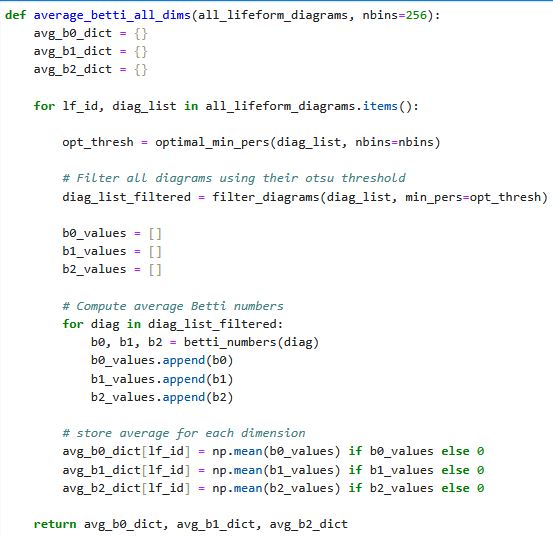
|
|
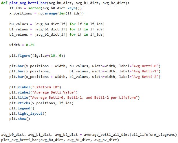
Which resulted in the following graph:
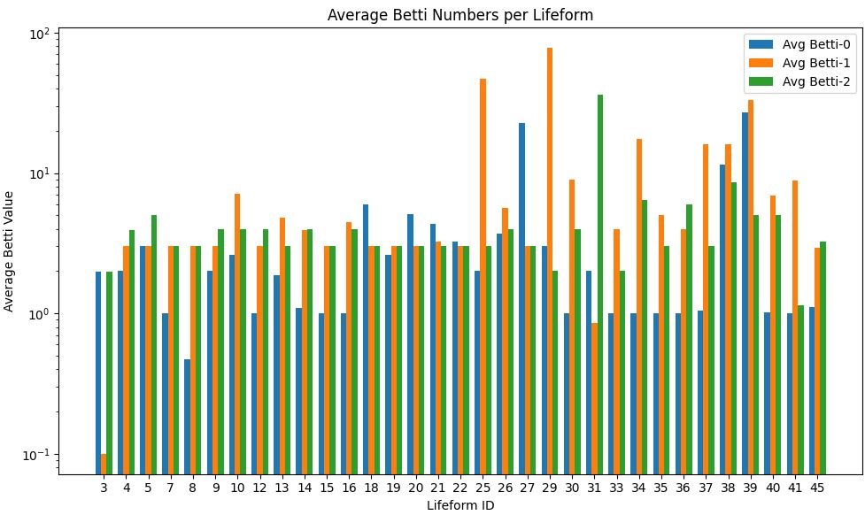
|
Including Betti-number evolution in animation
To get a better intuitive understanding for how the Betti numbers can be interpreted for a given lifeform, I decided to animate the Betti number evolution frame by frame by simply letting a vertical red line sweep through the Betti-number over time graph.
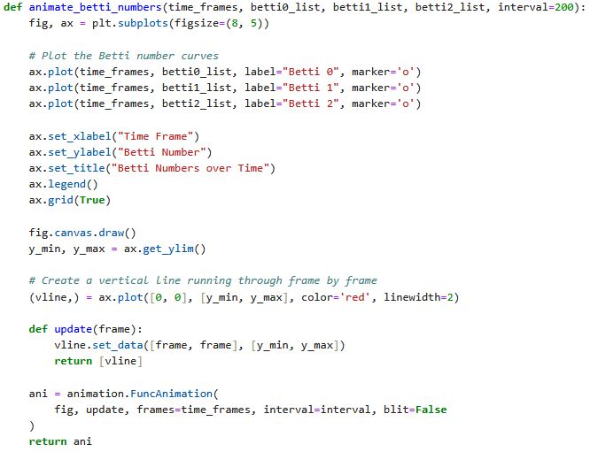
|
After describing the methodology, I will now showcase different examples of lifeforms and interpret the observations in the following section "Study of sample cases".