Modeling
of Phnom Bakheng
Part
3 – Working with Blender
written
by Christoph Hoppe
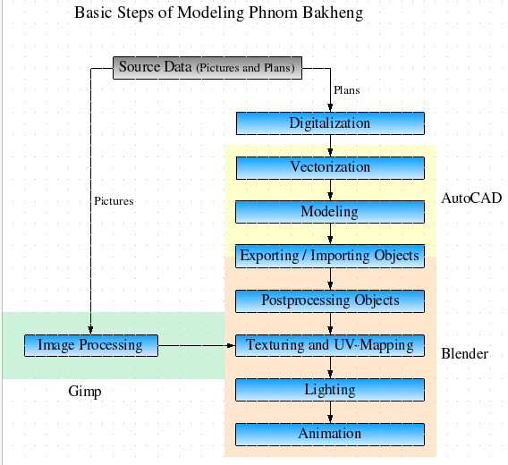
(fig. 1) This image shows the structure of our work, how it was organized.
The blue
rectangles stand for the production steps we needed to go through to
finish our work.
What this article is about
This article gives a short overview about the things, that I have been
working on. In the following, I will go through the steps of
creating a video sequence, after the objects were modeled in
AutoCAD. The software I used for finishing our work were the
open-source modeling and rendering environment
Blender and the open-source image processing software
Gimp.
The First Steps
When you take a look at fig. 1, we got at first some source data (grey rectangle). These were several
pictures taken with a digital camera and several scans of the old
plans, drawn by the french at the beginning of the 20th
century. For the plans, there follows a step I called
“Digitalization”, which means, that the plans needed to be
scanned and the scanned pictures needed to be “stiched”. The
plans were too big for A4 – format scanners, so they were scanned
several times in which the areas at the margin of these pictures
overlapped. Stiching means than, that from all pictures of a plan, one
big picture was generated, by comparing the overlapped areas and
generating a big picture with a special software.
This
was not part of our work, that's why it is not underlaid in yellow,
red and green, like the other steps.
The
first step of our work was to vectorize the plans. That means, that
we had to trace the drawings of the plans to make some sections of
polygons.
In the
next step, the modeling step, we made 3D objects of these sections.
For both steps see in Dong Wei's part for further details.
Although
I have been doing some modeling in AutoCAD too, the main part of my
work begins at exporting and importing models from AutoCAD to
Blender.
Exporting and Importing Models from AutoCAD to Blender
Our
first problem was, to choose an adequate data format for exporting our models from AutoCAD and import them to Blender.
We tried several formats and found out that the .STL format seemed to
be the best for both programs, because some of the
supported formats, such as .DXF, did not export and import all the
objects we wanted and sometimes misplaced or twisted the objects.
But
there is also one disadvantage of the STL format: AutoCAD is only
able to export one object at one time in a single STL-file, so we had
to export and import all objects separately.
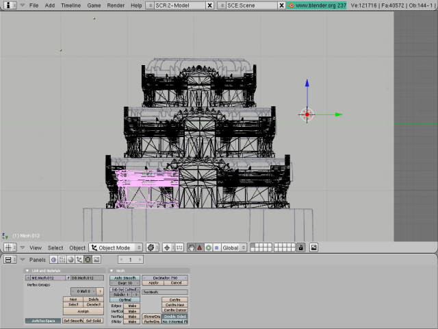
(fig. 2) A screenshot taken from Blender, were you can see some imported models in a wireframe display.
Only the bottom level was
modeled in AutoCAD, the two upper levels are just copies of this
level.
Postprocessing the Models in Blender
After
importing objects in Blender, we had to do some postprocessing work.
That was necessary because AutoCAD is still missing some functions
of 3D-rendering software. The function we missed the most was to
stretch objects along an specific axis. AutoCAD only allows to
stretch the object at its whole. We needed this function to generate
the upper levels of the towers. So we just modeled one level, copied and shrunk the bottom levels from the top of the towers and
copied and shrunk the levels lying upon this levels.
The
second function of blender we used for postprocessing, was its mesh
editing function. In Blender you can select specific edges or
vertices and draw these to any new position you like. We also used
this mainly for the upper levels of the tower, to adjust their the
shape to the available plans.
The
third function was the boolean operation function, i.e. substract,
addition and union operations for meshes. AutoCAD also provided us
these functions, but because it's famous for its accuracy, it often
displayed us errors than to simply union or substract us some
“solids”. This happens if the faces of the solids don't fit exactly together.
For
instance, the interior of the small towers was made in such way, that
we modeled the inner room as one filled mesh and cut it out from the
previously modeled objects with the substract function of Blender.
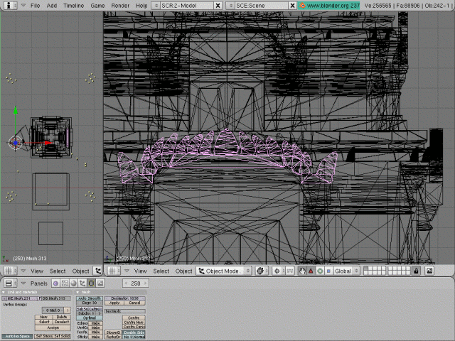
(fig. 3) Two screenshots were you can see how a pediment was stretched along the z-axis.
Once we
had finished this, the objects still look very boring, all gray in
gray with no colors and textures on them. This is
were the next step begins, the image processing part.
Image Processing with GIMP
As
I already told you, we were provided with lots of high resolution camera
shots. From these pictures we had to cut out the relevant parts and
adjust the colors, because they were taken under different lighting
conditions and sometimes just didn't look suitable for our models.
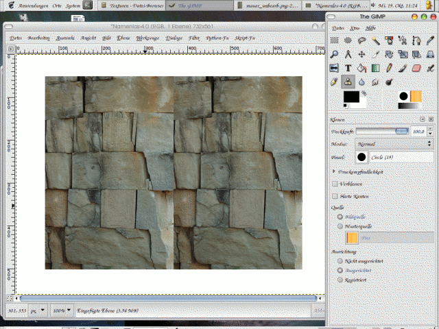
Another problem was to make the textures for walls and the floor
continuous. This problem rises up when a wall is longer than the
given texture. So the texture is repeated several times. As you can
see on the images, the edges of the texture itself don't fit
together, there are no seamless transitions between the edges.
With the
help of a so-called “clone brush” tool, we aligned these edges by
reconstructing the stones around them. This
tool just allows to copy a selected area and draws it to another
place with an adjustable opacity.
(fig. 4) Drawing over the edges of a wall texture with the clone brush tool of Gimp.
The red circle represents the source
area of this tool, the blue circle the destination area.
To
create an bumpy effect, when rendering these textures, we
finally created bump maps by desaturating the images (making them
grayscale) and inverting the colors. This works quite well, because
brighter areas on images are usually next to the viewer and darker
areas are a little bit farer away. And our images were taken at day
with natural sunlight coming from above and with no camera flash
light turned on.
(fig. 5) Screenshot from a rendering of an apsara (the texture
with the woman) showing which effect bumpmapping does.
This surface is
actually flat, only bumpmapping makes it look uneven.
There were still some other things we needed to do with the textures.
The problem was, that they were taken under different lighting
conditions and perspectives. Therefore, almost all had a different
color tone or brightness level. So we adjusted the colors, that
they fitted better together. Some images didn't have the right proportions, that's
because they were not taken directly in front of the temple but from
downwards, from the floor, looking up to the temple. We stretched these
images at one side (typically the upper side).
For all
these image processing steps, we used the open source software Gimp
(Gnu Image Manipulating Program), which met our demands to full
extend. After
editing the textures they needed to be laid on our models. This is
were UV-mapping starts.
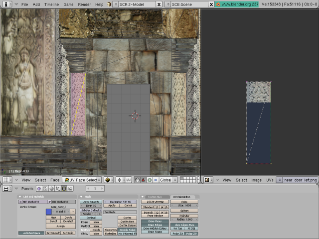
Texture Mapping - UV-Mapping
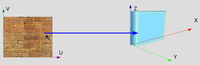
The UV stands for two texture coordinates,
which are positions within an ideal image (1:1). These typically
connect to points in a 3D mesh, to position an image texture on the
mesh. Like virtual tacks, they pin an exact spot on an image to a
point on an object's surface. Between the tacks, renderers will
stretch the image smoothly. This is what is referred to as UV
mapping.
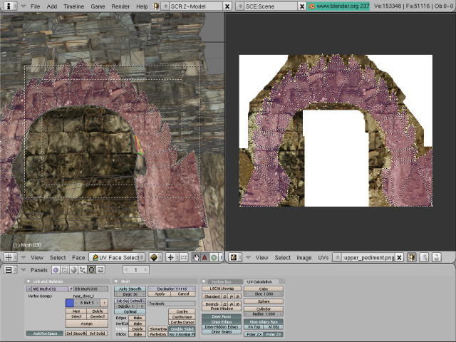
(fig. 6) UV-Mapping in Blender. On the right side, some kind of
template image is loaded and needs to be fitted with the polygons
selected on the left side.
(fig. 7) The same procedure shown with a pilar texture of the big tower
So our
work was to adjust the image source to fit correctly on the mesh. I
don't want to give you a Blender tutorial here, this would go beyond
the scope of this report. But you can see some screenshots here, that
you get an idea how this was done.
Lighting and Shadows
The
last step of our work was to choose and position the light sources.
We made several attempts with kind of different types of light
sources. Finally we came to the conclusion, that for our work, it was
the best to add an infinite light source, which casts parallel light
over the whole scenery.
For
rendering the shadows, we didn't used raytracing, because this needs
too much CPU-power and therefore is much too time-consuming. Instead
we positioned a light source of the type “spotlight” in the same
angle and position as the “sun”-light source.
Blender
allows to add light sources, which actually don't cast any light, but
only cast the belonging shadows. For these shadows we used the type
of the so-called “buffered shadows”, which are much more
quickly
rendered compared to raytraced shadows. This light source uses a
buffer, in which the non-illuminated regions are saved. So there is no
need to recalculate all the light paths for every frame as it would be
done by raytracing. Actually, the shadows don't look as exact as with
raytracing, but good enough for our purposes.
The
third light, also a light source of the type “sun”, lies
directly on the opposite side of the temple. For this light we lowered
the
intensity to about the half of our sunlight. This light was added to
simulate an ambient light. Without this light the casted shadows of
our spotlight were completely dark and didn't look realistic.
We
could have used radiosity rendering for simulating the diffuse light
casted from illuminated walls and objects, but this also needs too
much CPU-power and time for such a high-polygon scenery like our
temple.
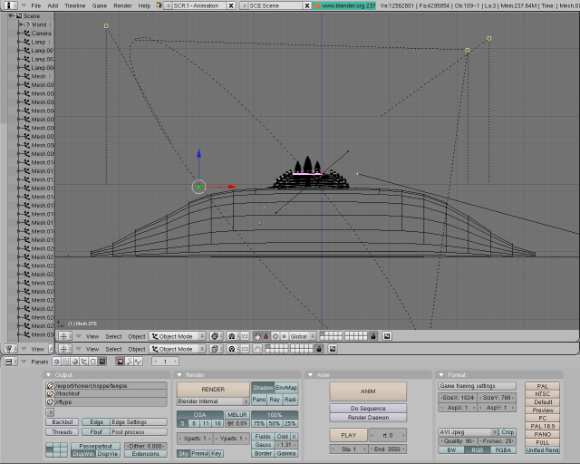
(fig. 8) On this screenshot you can see the position of the light sources and the light cone of the spotlight.
Animation of the Scene
The
last step of our work, the “animation” step, was comparably
simple to our previous steps. We just needed to make a camera flight
through and around the temple. Which means, we only had to move one
object, the camera, through the whole scenery. For
doing this, we needed to set different keyframe positions of the
camera.
In
the following, I will give you a small example how this was done.
Imagine, we are at frame 0 and our camera is placed far away of the
temple. We want to move the camera near the temple in 5 seconds. For
a smooth animation we need at least 25 frames/sec to be rendered. So
we go to frame 100, grab the camera, move it to a new position and
angle and save a IPO-keyframe. Now the camera moves in 100 frames from the first to the second position.
To
create an smooth animation, Blender uses so-called IPO-Curves which
interpolate between two IPO points. These curves are b-splines, of
which you can freely change the weightings with the help of the
IPO-curve editor of Blender.
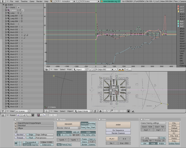
(fig. 9) At the upper section of this screenshot you can see the IPO-curve editor, in which each colored line represents
one coordinate in space (LocX, LocY, LocZ) or a rotation around the X,Y and Z-axis (RotX, RotY, RotZ).