1 Introduction

All digital measures can only record discrete data sets of reality. As the hardware gets more accurate and the amount of data gets even larger, it is more and more necessary to visualize it for a better understanding.

The process of visualization large data sets in 3D costs enormous computing power. In the case of laser scanning it is necessary to display the data sets in 3D, even on non-high performance computers like laptops.

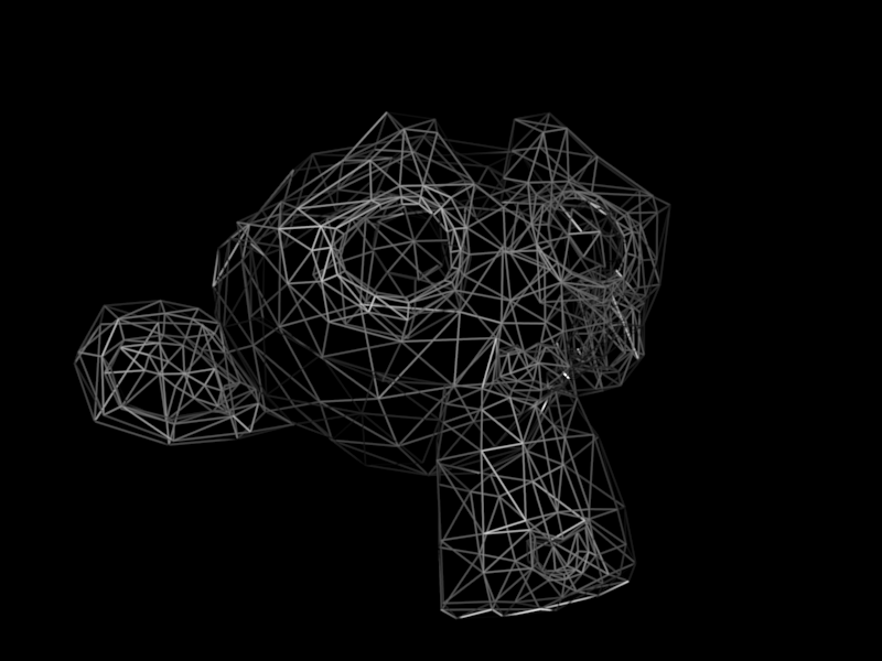
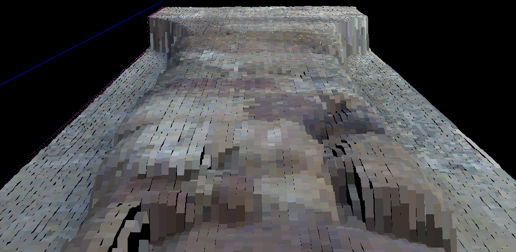
Our solution is to align a simple 3D surface to the existing data. While the amout of data will be significantly reduced, the properties of the scanned object, particulary the shape and color, will still be preserved.

1.1 3D-Laser Scanners

A 3D laser scanner is a device that analyzes a real-world object or environment to collect data on its shape and possibly its appearance (i.e. color). Many different technologies can be used to build these 3D scanning devices, each technology comes with its own limitations, advantages and costs. There are still some limitations in the kind of objects that can be digitized, because optical laser scanning technologies encounter many difficulties with shiny, mirroring or transparent objects.

Fig.1: The Callidus CP 3200 laser scanner.
Such a device aquired the data from the
Lorsch Abbey, which we used for testing
our algorithm. [1]

Applications:

• surveying (landscape, buildings, etc.)
• preservation of monuments, historic buildings and artifacts
• architecture (construction / reconstruction)
• scanning of objects and persons for 3D-movies and PC-games
• forensic securing

1.1.1 Basic Functionality

• An extremely short laser pulse is emitted by the scanner, hits an obstacle by which it is reflected, and is then received again by the scanner. The measured time of flight is proportional to the distance between scanner and object
• The applied laser type allows measurements independent from ambient light

Fig. 2: The left drawing shows the rotation angle of the scanner from the top view. The right one the rotation angle from the side view. It is obvious that the shadowed area on the floor is dependent on the installation height of the scanner. [1]

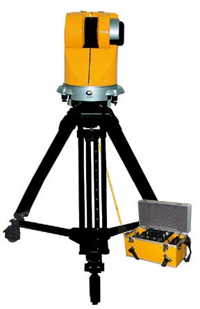
During the measuring procedure, the laser scanner integrated in the measuring head rotates by 360° along the horizontal plane. By means of a rotating mirror, the laser beam is emitted in the shape of vertical fans and thus covers of 140° of its environment in the vertical plane.

With a CCD-camera integrated in the system, it is possible to record panorama or detail images that are available for documenting the scanned object. These pictures deliver a template to automatically assign the true colors to the recorded point sets.

1.2 Point Clouds

A 3D point cloud is a discrete set of three-dimensional points. The coordinates of these points are calculated from the angles and the distance to the scanning device.

We used the two following kind of formats to store these data sets:

1.2.1 Supported Data Formats

VRML-2.0

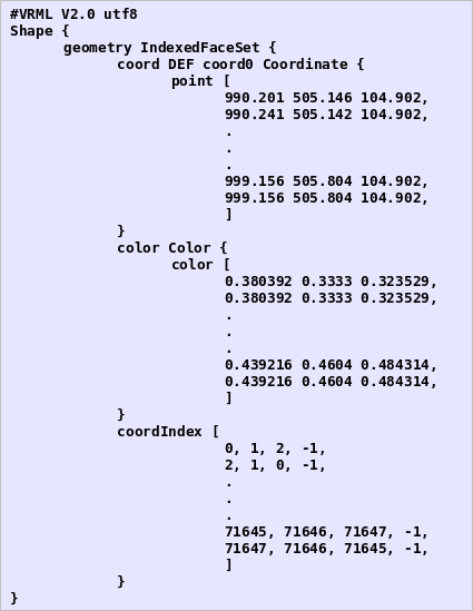
While working with point clouds, we only need to store the three coordinates for each point and the according color as RGB values.

We have chosen the IndexedFaceSet geometry for storing our data, because it is easy possible to extend it to a fully meshed 3D-model.

The drawback of this format is that coordinates, colors and the mesh data are stored consecutively in the file, which leads to a suboptimal processing time.

Fig. 3: A cutout from a VRML-file we used for storing a laser
scanned point cloud and the generated mesh.

ASCII-TXT

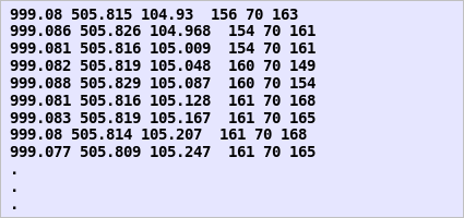
In this format we save the coordinates and the according RGB-colors each with a single line. The benefit from this method is that it needs only half the disc space and processing time.

The only disadvantage so far is that there is no meshing saved, so it is currently only appropriate for point clouds.

Fig. 4: A cutout from a text file we used for storing a laser
scanned point cloud.

2 Meshing of Point Clouds

2.1 Meshes

 

Fig. 5: A wire-frame rendering of a triangle mesh created with the 3D-modeling and rendering application Blender.

mesh (engl.): "In the computer graphics representative for a polygon network for modelling 3D objects'' [2]

Why meshing point clouds?

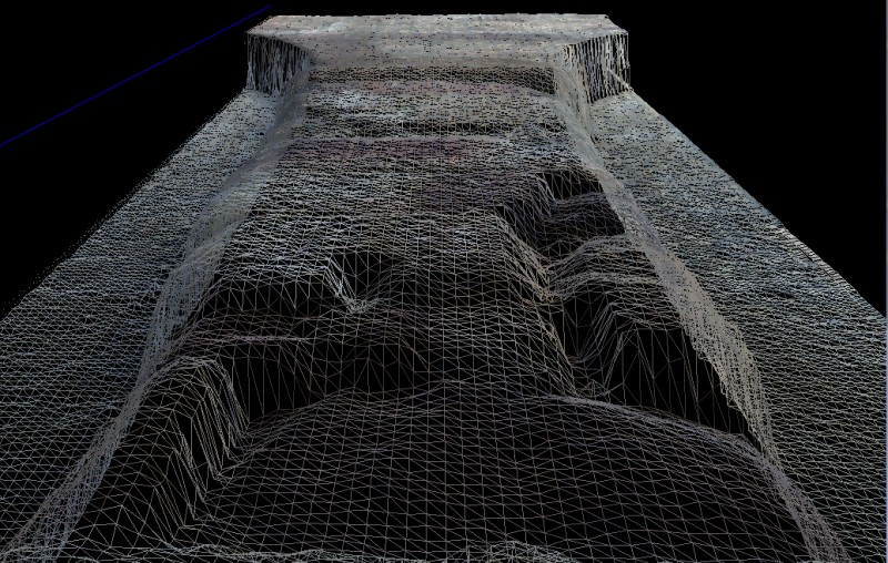
Modern 3D-graphic cards are not optimized for rendering point clouds but displaying triangles and triangle meshes.

Therefore meshes offer an enormous speed advantage in regard to point clouds and make a smooth illustration of complex surfaces and structures possible.

2.2 Triangulation

"A triangulation of a set of points P is the triangulation of the convex hull of P, with all points from P being among the vertices of the triangulation." [2]

The naive start to create a mesh is to triangulate the point set, i.e. to connect all points to triangles respectively a triangle net.

This method has several drawbacks:

• calculation speed
• memory usage
• instability to outliers
• no smoothing of the surface
• scalability

That's why we have chosen to go a different way as described in the following chapter.

2.3 A Basic Approach for Meshing Point Clouds

1. Choose a suitable orthographic projection of the point cloud
2. Starting from a chosen point:


3. Find all points within a squarish area of a predefined size
4. Calculate mean height and mean color of all these points
5. Fit two triangles to the vertices of this area
6. Delete all points inside the area
7. Move area
8. Goto 3. until no points left

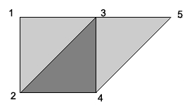
For moving this square along the surface, we chose a bottom-up translation, i.e. starting from the selected point we move the square upwards along the point cloud, until no more points are found. Then we move it one of its size to the side and back to the bottom and so on, until the whole surface is covered with triangles.

Fig. 6: Bottom-Up translation in 2D

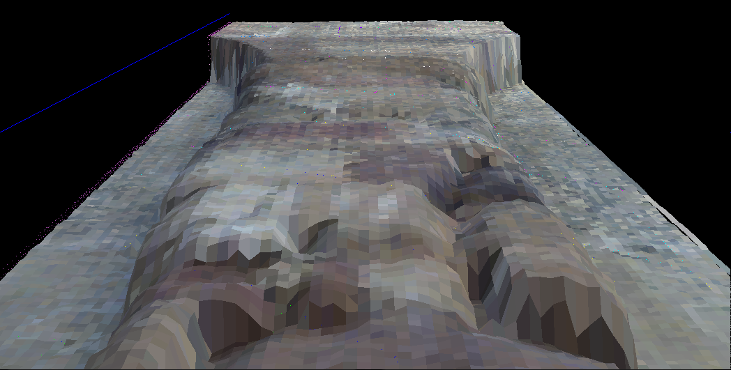
In the second step, to create a closed mesh, it is mandatory to connect the created strips. Therefore the mean value for the height of two super-imposed vertices respective to the orthographic projection area has to be calculated. The triangles get rearranged according to this value, which closes the gaps between two adjacent strips.

Fig. 7: This animation illustrates the fundamental principle of our meshing algorithm. It is based on screenshots directly taken from our software PointMesh.


Fig. 8: A meshing result from PointMesh with a square size nearly to the original scanning resolution. The created triangle strips are still unconnected.


Fig. 9: The same mesh as above after connecting adjacent triangle strips to each other.


Fig. 9: A wire-frame view shows the high detail level of the generated mesh.

2.4 Our Globefish-Algorithm

The most time-consuming part of the algorithm was the identification of the points within the square necessary for the calculation of the mean height and color, so the triangles could be aligned to the surface of the point cloud. It was necessary to divide the given data set into several parts to achieve a good performance. The separation algorithm is based on sorting the points according to the euclidian distance to the starting point. So far the space gets partitioned into 10 equidistant spherical shells (that's why we've chosen the funny name Globefish for it). This partitioning results in a remarkable speed advantage because not the whole array of all points has to be traversed in order to find the points lying in the square.

Fig. 10: A point cloud partitioned into ten spherical shells marked by different colors.

2.4.1 Comparison to a Naive Algorithm

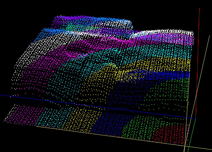
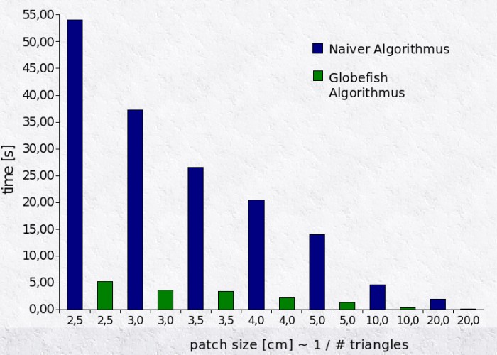
Fig. 11: This diagram shows a speed comparison between the Globefish and a naive (non-separated data array) algorithm.

In this test we used a relatively small file and varied the size of the square (patchsize). The speed-up factor lies here at 10x and between 4x to 6x in the average case for larger point clouds.

2.5 Problems

• Because the algorithm has a static projection area, an accurate meshing is only possible up to 45 degrees to this section. An angle above that value leads to loss in the surface details.
• The patch size is constant. It can be changed before the algorithm starts, but cannot be changed during the process. This aspect has a lot potential of speeding up the whole meshing process. For example, it is not needed to render a flat wall with 1000 triangles, so if the algorithm could change the patchsize respectively to the shape of the surface, it would lower the runtime dramatically.

2.6 Future Prospects

• There is a lot room of improving the performance. Things like a handy separation of the data or a clever sorting of the points are only a few ways to go.
• The projection area is fixed during the runtime, it would be a great improvement to make it automatically rotateable by the algorithm. So a closed room or an individual object could be meshed in one run.
• Embedding a level-of-detail (LOD) algorithm would offer the possibility of deleting unnecessary triangles from the created mesh.
• Extracting textures from the mesh and mapping them on such a reduced model would offer a lot of possibilities.

3 References

• [1]: Images (c) Callidus Precision Systems
  
  http://www.callidus.de
• [2]: http://en.wikipedia.org/wiki

• GLUI - A GLUT-Based User Interface Library (P. Rademacher), 1999, http://www.cs.unc.edu/~rademach/glui/src/release/glui_manual_v2_beta.pdf


• OpenGL(R) Programming Guide, 1999, (M. Woo, J. Neider, T. Davis, D. Shreiner)


• Level of Detail for 3D Graphics (D. Luebke, M. Reddy, D. Cohen, A. Varshney, B. Watson, R. Huebner), 2003, Elsevier

Example Results