Animation and Simulation of Infectious Diseases

Software Practical by Sonasha Auer Wilkins
Supervised by Dr. Susanne Krömker

Motivation

Modeling infectious diseases helps us improve our understanding of certain characteristics such as the speed with which it can spread in a population, the critical immunization threshold needed for it to die out or the number of deaths that can be expected from an epidemic. 
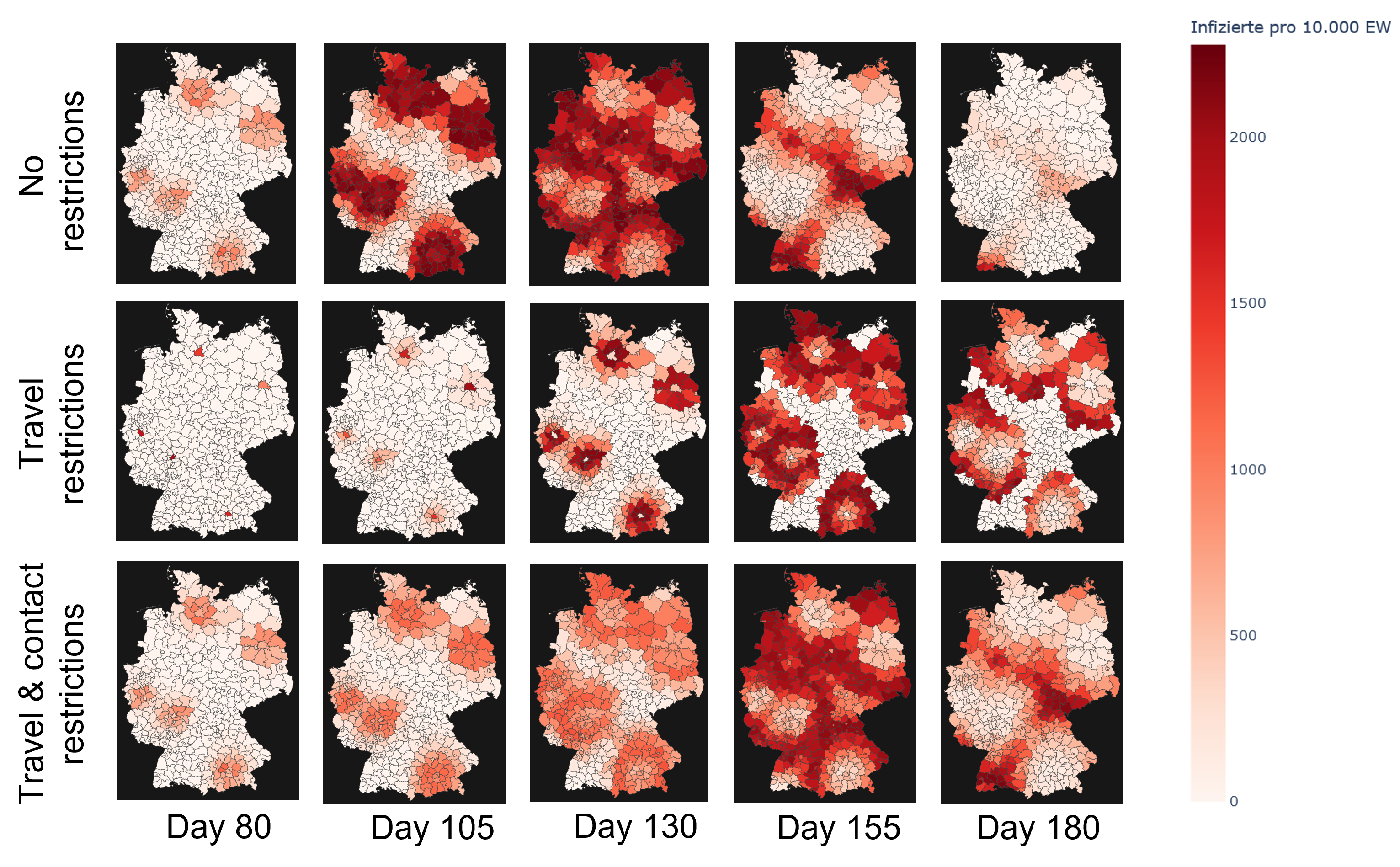
Additionally, we can evaluate the effectiveness of preventive measures such as quarantines, contact and travel restrictions or targeted vaccination campaigns.
Models generally only represent a simplified view of the often complex real-world situation, where the spread of a disease can be influenced by a populations age, the economic wealth of a region, the complex web of cantact between individuals or seasonal variations. Especially in the case of new viruses such as Covid-19, many values needed for accurate modeling are yet unknown due to a lack of data. Even though it might be possible to fit the parameters of a model to the known data of a disease, the correctness of these parameters can not be guaranteed.
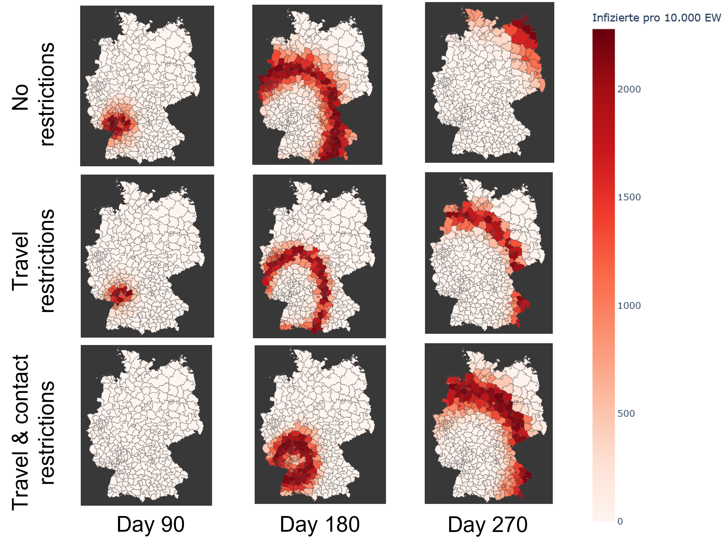
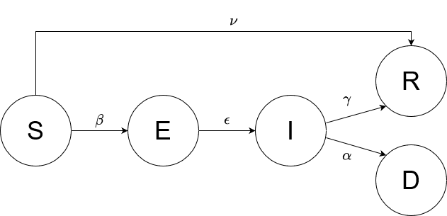
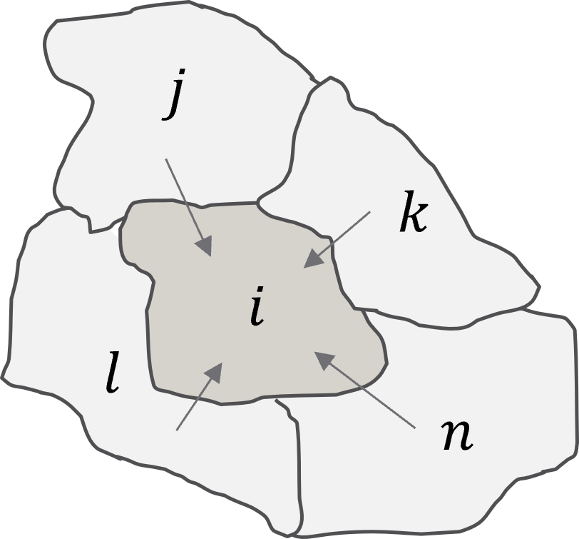
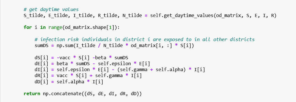
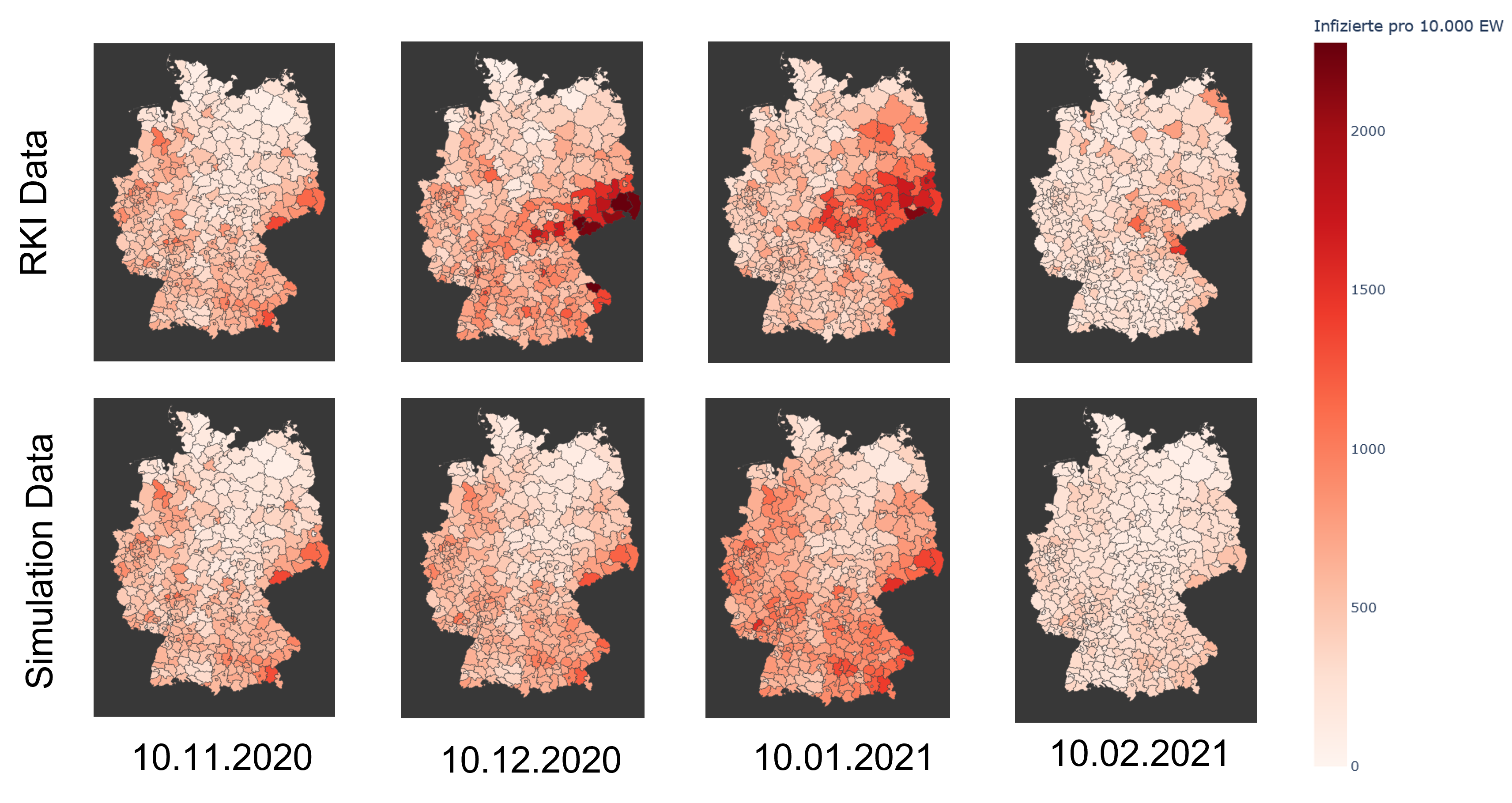
In this practical project, a SEIRD compartment model is used to evaluate the spread of an infectious disease 
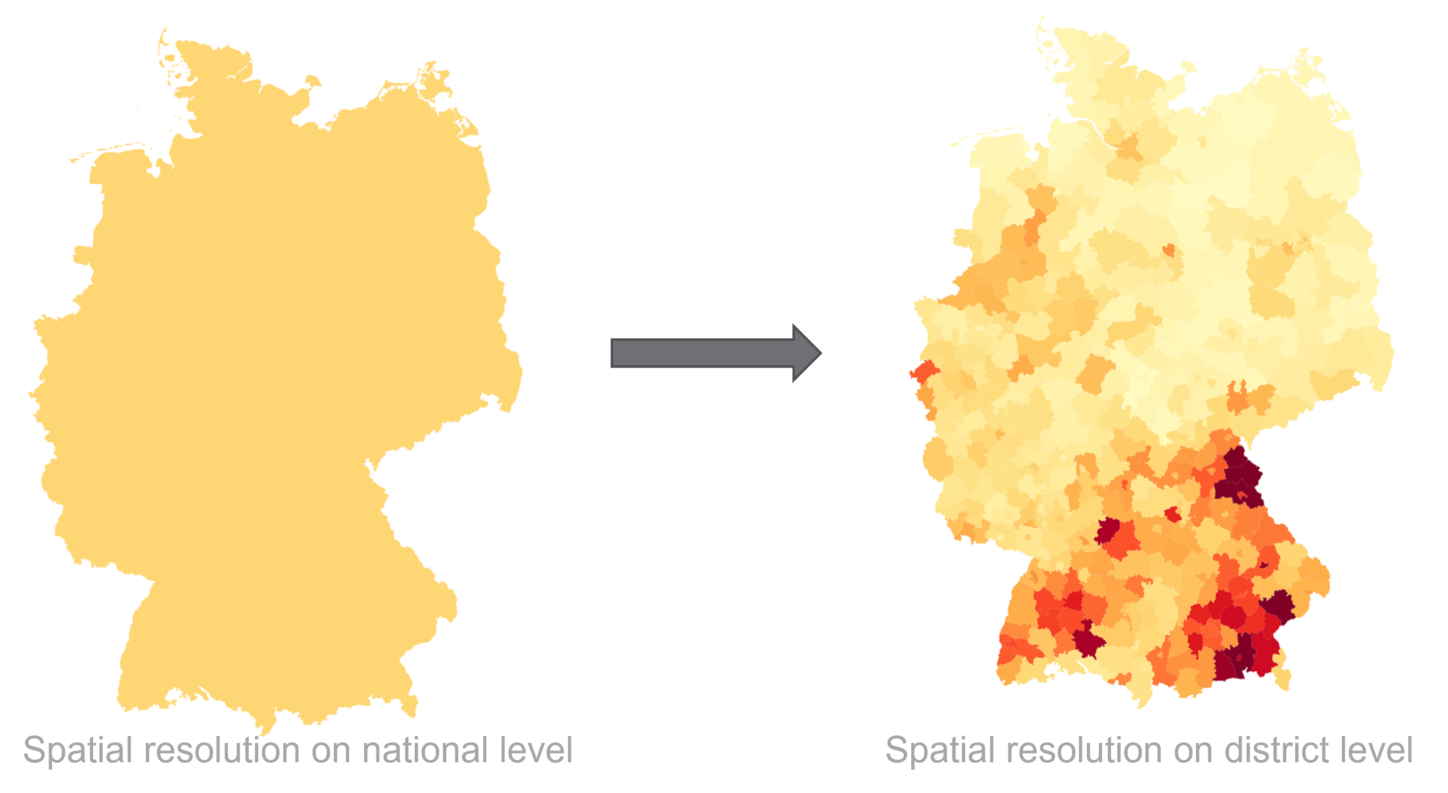
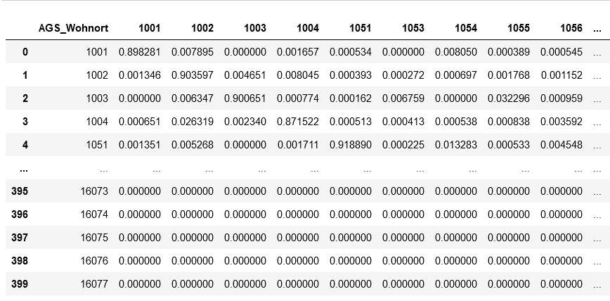
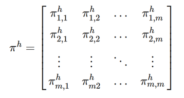
using the example of Covid-19. In addition to the temporal aspect of compartment models, a spacial aspect is 
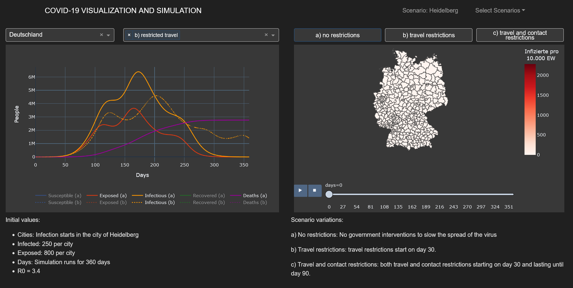
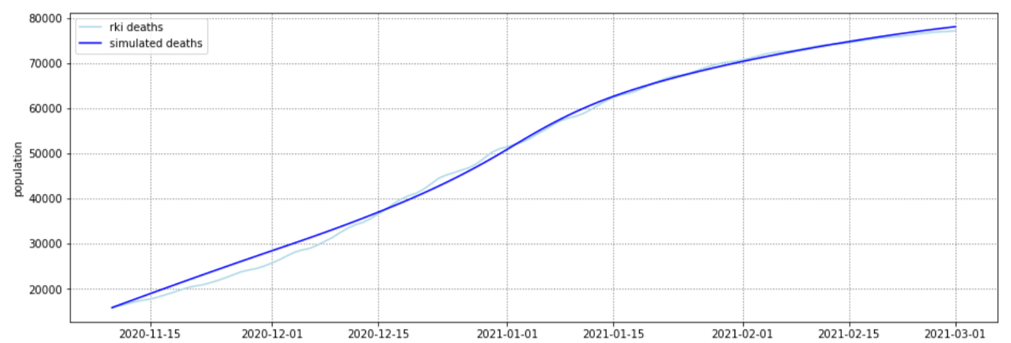
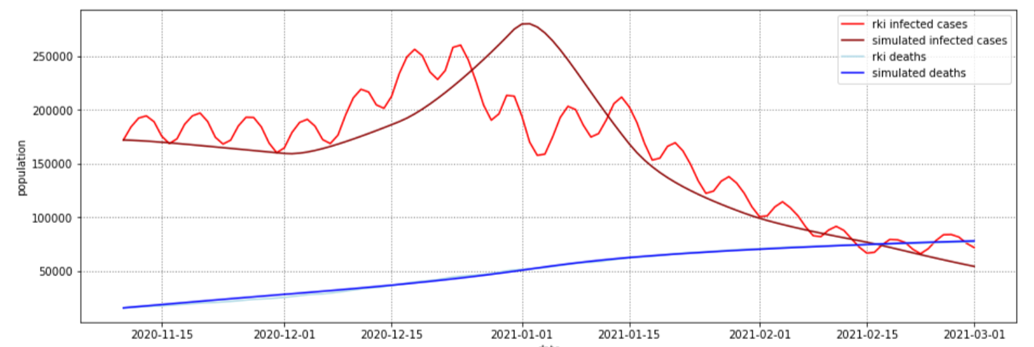
added by incorporating interregional commuters into the model. The results of the model were animated and a dashboard was implemented for presenting the visualized results.

The implemented model as well as the results are discussed in the following sections.

Compartment Models

Compartment models are a mathematical modeling technique dating back to the early 20th century. The main idea lies in dividing the population into labeled compartments representing different states an individual can find themselves in, and allowing people to transition from one compartment to another at given time rates and in specified directions. For infectious diseases, the compartments typically include a group of susceptible individuals (S) wo have not yet been infected, the infected individuals (I) who can spread the disease to others and the recovered individuals (R), who are no longer infectious and are assumed to be immune. Many variations of this simple SIR model exist, with additional compartments and transition rates between them. The models can therefore be adapted to different diseases and become arbitrarily complex.
Compartment models are typically solved using systems of ordinary differential equations (ODEs), which capture the dynamic change of each group over time. The differential equations can be either stochastic, meaning the results are based on probability and may vary each time the model is run, or deterministic, meaning the results are pre-determined by the model parameters and remain the same with each run. For this project, deterministic ODEs are used.

SEIRD Model

The SEIRD Model is a compartment model which contains the following groups:

  • S - Susceptible: people who can still become infected with the virus
  • E - Exposed: people who have been exposed to the virus but are not yet infectious
  • I - Infected: people who are infectious
  • R - Recovered: people who are no longer infectious and have immunity
  • D - Dead: people who have died of the virus
  • (V - Vaccinated: people who have immunity due to vaccination, subgroup of Recovered)

The model parameters determine the rate with which people transition from one compartment to another. For the SEIRD model, the parameters are as follows:

  • β - Transmission rate: the rate at which people become infected (probability of disease transmission multiplied with the average contacts per person per time step)
  • ε - Incubation rate: the rate at which people become infectious after being exposed to the disease
  • γ - Recovery rate: the rate at which an infected person becomes no longer infectious
  • α - Death rate: the rate at which people die from the virus
  • ν - Vaccination: the rate at which people are vaccinated

The system of ordinary equations for the SEIRD model calculates the rate of change over time, measured in days. For each equation, people are removed from one compartment and added to another at the corresponding rate.

Based on the transmission rate and the recovery rate, the reproductive number can be determined as R = β/γ, which represents the average number of people one infected person will infect. This value is important for determining the spread of an infectious disease in a population. If R < 1 is true, the disease will die out, if R > 1 is true, the disease will spread in the population. The basic reproductive number R0 is a constant value for each infectious disease and represents the number of people an infected person will infect assuming a population where everyone is susceptible to the disease. The effective reproductive number Re on the other hand represent the number of people one infected person may infect assuming the population can also be immune and incorporating preventive measures by the government. This value can change from day to day and also varies in the model, depending on the current transmission rate β.

The Spatial SEIRD Model

Traditional compartment models treat the population as homogeneously mixed, meaning that each individual has the same probability of coming into contact with any other individual in the population. However, in reality human interaction contains a spatial aspect which plays a role in disease spread.

Inspired by the paper Simulating the impacts of interregional mobility restriction on the spatial spread of COVID-19 in Japan by Keisuke-Kondo, the implemented SEIRD model changes the resolution from the national to the district level and includes a spatial aspect by modeling interregional mobility across district borders. The data for interregional mobility was derived from location data of mobile devices, however, since such data is not accessible in Germany, commuting statistics between districts was used instead.

Excerpt of the OD matrix for German districts

Modeling Spatial Mobility

The mobility across district borders is modeled using an origin-destination (OD) matrix. This matrix πh with h ∈ S, E, I, R, contains values πij representing the probability of a person in region i to commute to region j during the daytime:

We set πS = πE = πR to model unrestricted travel between districts for individuals in the corresponding compartments S, E and R. For infected people we set πI = I (identity matrix), since they are assumed to stay home while they are infectious.
The probability values were derived from statistics provided by the Bundesargentur für Arbeit, and were converted from separate Excel sheets into one 400x400 Pandas DataFrame. The commuting data of each district was restricted to a 150 km radius in order to filter out unlikely outliers such as commuters traveling from Heidelberg to Berlin on a daily basis.
The population flow between districts can then be modeled for each compartment as the probability of commuting from district i to j at time t:

Therefore, the total inflow of people from all m districts into a district i is given by the following equations:

Spatial System of ODEs

For the spatial model, each district has its own internal SEIRD model, which assumes the population is homogeneously mixed. Spatial spread of the disease is incorporated with the OD-matrix representing the commuting population across district borders. People who commute from district i to district k are exposed to the total amount of infectious individuals in district k during the daytime. The disease therefore has two possible ways of spatial spread: it can be contracted in the region of work and brought home by commuters to their region of residence, or it can be contracted in the region of residence and brought to the region of work.
This spatial aspect is incorporated into the transition rate between the susceptible and exposed compartments by calculating the sum over all susceptible people who commute to a different region during the day, and the total inflow of infected people into those regions that they are exposed to. The rest of the ODE system looks similar to the previous SEIRD model, except that now we have one model for each district i.

Model Assumptions

  • Spatial mobility: only the movement of commuting workers is considered in this model. In reality, a population's movement is far more complex. One could include random movement into the model to account for this

  • International borders: the commuting statistics used for the OD-matrix does not include data about international commuters. This means that districts bordering on other countries do not reflect the actual work-related inflow and outflow of people

  • Virus mutations: this model does not include any virus mutations, which might affect the transmission rate and the virus induced death rate

  • Population demographics: the population is assumed to be constant, meaning there is no population growth due to births or immigration. These factors can be included in some SEIRD models, however the importance of including such factors depends on the disease that is being modeled

  • Immunity: recovered and vaccinated people are assumed to be entirely immune to the disease. In certain cases, including COVID-19, people can lose immunity at a given time rate or become infected with different strains. This can be modeled by moving people from the recovered back to the susceptible compartment at a given time rate

Implementation

Excerpt of the SEIRD model implementation in Python

Model implementation

The system of ordinary differential equations was solved using the Scipy library. The Scipy odeint function uses the Adams method for solving the ordinary differential equations numerically. The values for each district are concatenated into an array and extracted in the model in order to calculate the change for each compartment from one day to another. On average, solving the model for a time period of 360 days takes 20 seconds.

The starting values for the model can either be set to simulate a specific scenario or to reflect a real-world situation. For scenarios, it is required to define the number of infected and exposed people for certain districts (at least one infected person is required), while the real-life scenario requires a date which lies inside the time period of the Covid-19 pandemic. The initial values of the compartments can then be derived with the following formula:

,

where

  • Ti(t): cumulative deaths reported in region i up until day t
  • Pi(t): cumulative positive cases reported in region i up until day t
  • γ-1: infectious period in days
  • ε-1: incubation period in days

Once the model has run through, the data is parsed into a Pandas DataFrame which can be further processed for visualization.

Parsing Covid-19 Data

In order to compare the model to real world data, values of the Covid-19 pandemic in Germany were used. The data was taken from the Robert Koch Institute (RKI) using the Arcgis REST api , and includes the entire history of the pandemic for each district. This data required some pre-processing including summing up the data for all districts in Berlin which are counted separately and parsing dates. Additionally, the one-week incident number (7-Tage Inzidenz) is calculated as well as the average infected per 10.000 citizens.
The result is a dataset containing all values for each district from the beginning of the pandemic until now (about 37 MB). This dataset is updated whenever it is loaded to include the new data uploaded by the RKI.

Visualization of Spatial Data

In order to visualize the spatial data a choropleth map of Germany on district level is created using a geojson dataset containing polygons for each district (Landkreis). Since there are 400 districts, rendering the data can be slow, however, this can be optimized by simplifying the polygons and converting the vertices arrays to Numpy arrays. Some polygons need special handling, such as the district of Eisenach, which must be dissolved as its status was changed so that it no longer counts as a district.
In addition to the geojson file, information about each district is required, such as the name, population, and the identifying key. This information was taken from the Destatis Organization and parsed into a Pandas DataFrame.
Using the Plotly library, we can then create an animation by linking the polygons to the county metadata and the disease values for each district at the given timesteps.

Results

, , ,

Comparison to RKI Data

The spatial SEIRD model can be compared to the RKI data by running the model with the same initial values as the real pandemic showed on a chosen date. This date was set to the 10th of November 2020, which marks the beginning of the second Covid-19 wave in Germany.
After creating the initial values as described previously, the model parameters are fit to the RKI data of accumulative deaths, since these values more reliably reflect the true nature of the pandemic than the number of infections can.
The resulting parameters are as follows:

  • R0: 3.4
  • ε: 0.191
  • γ: 0.1
  • β: 0.34
  • α: 0.0036

Using these parameters, it can be seen that the modeled infected values provide a good approximation of the RKI's data on infection cases during the second covid wave.

In order to make the previous comparison, the values per compartment and district were summed up to give us nationwide results that approximate the true RKI data. Looking instead at the district level spatial resolution, we can visually compare the model to the RKI data by plotting the values on a choropleth map.
Here we see that even when the nationwide values approximate the true values, it is quite difficult to capture the local behaviour of infection dynamics. This is largely due to the far more complex interactions between people in the real world compared to the simple commuting population in the model.

,

Scenario: Outbreak in Five Cities

For this scenario, the spread of the virus over 180 days is modeled using five starting points in Germany's largest cities: Berlin, Hamburg, München, Köln and Frankfurt.
Each city has the starting values:

  • E: 100
  • I: 50
  • R0: 3.4

Three different scenarios were modeled:

  1. No restrictions: the model runs through with the initial values
  2. Travel restrictions: the OD-matrix is replaced with the identity matrix on day 2, meaning traveling between districts is no longer possible
  3. Lockdown (Travel and contact restrictions): three week travel and contact restrictions starting on day 90. Here, the identity matrix is used and the transmission rate β is scaled down so that we receive an effective reproductive number Re = 0.8

Looking at the results of the modeled scenarios, we can see that travel and contact restrictions push back the outbreak by the duration of the lockdown. The state of German districts on day 155 for the lockdown scenario looks similar to day 130 in the no restrictions scenario.
Similarly, the spread of the virus is reduced in the travel restriction scenario, however here people in certain regions are exposed to a higher infection risk, due to the population not being "diluted" by an inflow and outflow of people from different regions.

Scenario: Outbreak in Heidelberg

For this scenario, we model the spread of the virus over 360 days with the starting point in the city of Heidelberg.
The starting values for this scenario are:

  • E: 800
  • I: 250
  • R0: 3.4

Similar to the previous example, three different scenarios were modeled:

  1. No restrictions: the model runs through with the initial values
  2. Travel restrictions: the OD-matrix is replaced with the identity matrix on day 30, meaning traveling between districts is no longer possible
  3. Lockdown (Travel and contact restrictions): two month travel and contact restrictions starting on day. 30 until day 90. Here, the identity matrix is used and the transmission rate β is scaled down so that we receive an effective reproductive number Re = 0.8

This scenario shows the circular spread of the virus starting in Heidelberg and moving outward. People in the center of this circle have already contracted the virus and are now considered immune. The different scenarios show similar results as seen in the previous example, namely the slowing down of the virus spread through contact and travel restrictions.

To make the effects of restrictions more visible, we can look at the graphs of the model results. For the values of Heidelberg's district, we see that the highest peak of infections is given in the scenario of travel restrictions, which exposes the population to a higher infection risk inside the city. Since the lockdown scenario has a reproductive number smaller than one, the number of daily infection cases begins to reside during the phase of travel and contact restrictions. The peak of infected people is pushed back by two months and also shows lower values by about 5.000 people.
Comparing this to the nationwide number for the same scenarios, we can see that travel restrictions, which caused a higher peak in Heidelberg, reduce the nationwide numbers by the largest amount (from about 6.4 million to about 4.6 million). The two-month lockdown however only pushes back the peak by the same time period and does not result in a notable reduction of infected people.

Dashboard

To demonstrate the results of the model, a dashboard was constructed using Plotly Dash. This dashboard has several pages for the two scenarios and the RKI comparison. On the left side one can view a graph which shows the numbers of each compartment during the chosen time period. One can either set this graph to display the nationwide cases or specify a district. Additionally, it is possible to compare different scenarios of restrictions to each other.
On the right side, the animation of the infected cases can be viewed. By hovering over districts, one can see the district name as well as the current number of infected people.