Home Gitlab Repository Planet Generation Planet Gamification Simulation Presentation Contact
No Planet B

No Planet B

No Planet B is the result of a masters practical in the Field of Computer Science under the supervision of Prof. Dr. Suanne Krömker, conducted at Heidelberg University in the winter term of 2021/22. Authors are Johannes Bohlig and Dominik Buchmann. The focus of this practical was to develop a video game capable of serving as a complex simulation with respect to the energy supply and demand of a procedural generated planet and its population. The main parts of this work are given in the planet generation and simulation. Both are described in detail in the following sections. We used the Unreal Engine 4.26 to develop the simulation and organised our work via Gitlab.

Planet Generation

MainCycle

MainCycle

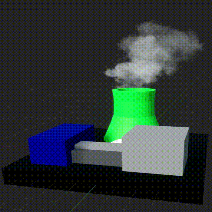
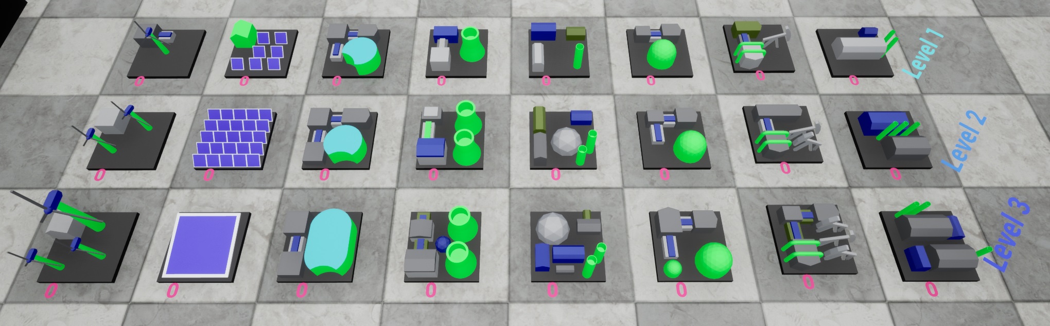
As basis and playground for the game serves a procedually generated planet. To accomplish that multiple steps are neccessary. 
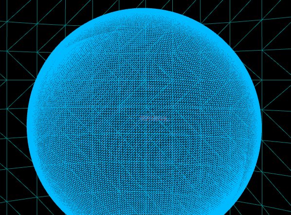
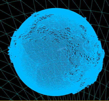
The initial shape of the planet is a flat sphere. This sphere has multiple requirements to fulfill:
- it has to consist of many manipulatable vertices
- these vertices should be distributed as uniform as possible
- the vertices have to form a continous mesh

To meet those requirements in the first step the vertices are created and placed uniformly in the shape of a cube. Those vertices are also stored in a 1D array and serve as logical and visible mesh. After the cube is created it has to be shaped into a sphere. Therefore a formula is used to calculate new point coordinates based on their cube position and relocate them. This could be done by just normalizing the lengths of the points vectors, in this project we chose a more precise way by using this formula:

x = x*sqrt(1-(y² + z²)/2 + (y²*z²)/3)
y = y*sqrt(1-(z² +x²)/2 + (z²*x²)/3)
z = z*sqrt(1-(x² + y²)/2 + (x²*y²)/3)

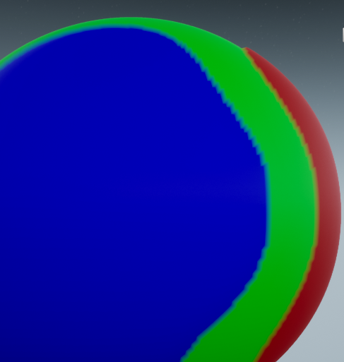
After successfully creating the sphere we have to form landmasses. Therefore a noise function, the so called "3 Dimensional Perlin-Noise" was used, which is ideal to transform surfaces into landscapes. To form mountains out of continents the Perlin-Noise transformation has to be done twice, the second time on top of the landmasses formed by the first transformation. In order to render the resulting mesh, it has to be triangulated. Therefore quad cells are counted in 2 orders:
- top left, top right, down left
- down left, top right, down right

Since the points are already vectors in outer direction they are also used as surface normals. The UV coordinates are created by transforming the point coordinates to longitude,latitude coordinates and map them onto a longitude by latitude texture.
This planet generation based on the Unity-Series of Sebastian Lague
Youtube Playlist

Planet Gamification

Requirements

The created planet has to be transformed into a playground. Therefore requirements have to be fulfilled:
- Classify cells (Water, Land, Mountain, etc…)
- Create continuous Surface
- Identify Continents on the surface
- Interact with the planet, continent and cells
- Need to move objects seamless on the surface

Cell Classification

To differentiate between different kinds of planet areas, the surface has to be classified into classes. There are three classes we differentiate into:
- Water
- Land
- Mountain
The classification is done by height meisure of every vertice, where the height is the distance of the vertice from the planet origin. In the first step we have to find out the maximum height of all vertices. With the maximum distance we can now do the classification: Cells with height: - under 1/3 of the maximum height are classified as Water
- between 1/3 and 2/3 of the maximum height are classified as Land
- over 2/3 of the maximum height are classified as Mountain
After the classification vertices of the water and land classes get leveled. All "Water-Vertices" get leveled to height 0, all "Land-Vertices" get level to the height 0.5*maximum height. Mountains maintain their different height levels to let them appear rough.

Continous Surface

As mentioned in the planet generation, all vertices are stored in a 1D-Array. Those points are also called "cells". In this game we want to be able to move from every cell to another seamlessly. Therefore the surface has to be continuous.
To achieve this the "Borderless-Array-Access" and "Borderless-Index-Map"- Methods were developed. These methods contain a static mapping consisting of cube side offsets and turning angles.
The offsets are neccessary since we want to map from one cube side to another, by adding an offset to the index in the 1D-Array. Turning angles are needed to turn the index counting direction, since the index directions of different cube-sides, relative to another side are diverging. With the offset and direction applied to the calling index of one cell, we can reach every other cell of an adjoing cube side and get an continous surface.

Identification of Continents

To identify the continents and islands created by the noise on the sphere, make them logically seperatable and store them as disjunct objects, a method is needed. For this purpose the "Continent Creation Algorithm" was developed in the scope of this project, which consists of 3 stages. In the first stage Every cell of the planets surface is traversed by an 3 x 3 matrix line by line. With this matrix the cells get a number assigned based on their classification. - -1 if it is classified as Water
- a positive number if it is classified as Land
A special case happens, if a cell in the kernel has already a positive number. Then the current cell is saved as a pair with the (lowest) number in the kernel, because they belong to the same continent, e.g. {1,2}. The numbers which will be assigned to the cells are based on a "polygon-counter". The counter is always increased by 1, if the classification of cells changes from land to water. This means, that the border from a continent is reached and the continent is left. To cover edge cases of the surfaces, where the matrix on one of the sides of the cube laps onto another, the "Borderless-Array-Access" is used. The first stage results in many associated pairs of polygon-pairs.
In the second stage the found polygon-pairs of the first stage have to be combined to find further associations, which means the found associated continent pieces will be associated if they are connected. There are 3 different cases where associations can be found:
- Case 1:
Pairs that are found by the kernel in stage 1 and have the same first value
{1,2} ; {1,3} => {1,2,3}

- Case 2:
Pairs or associations that have their first pair value in as a second (or higher) value
{1,2}; {2,3,4} => {1,2,3,4}

- Case 3:
Pairs or associations that have a different first value but same second value
{1,4};{2,4} => {1,2}

All of the associations have to be made seperately, as long till no changes can be found anymore. To enhance the performance of the algorithm, the array iteration happens from back to front, since we want to minify all numbers.
After all associations have been found in stage 2, the final stage 3 happens, where the minified numbers get assigned to the continents as IDs. The IDs enable to call continents and use them as disjunct objects. Finally continents get colored depending on the value of their ID, to also seperate them optically from one another.

MainCycle

User-Planet Interaction

To make the planet interactable and clickable with the mouse another method has to be developed, since the Unreal Engines collision detection can't be utilized due to the sheer mass of collision objects and the resulting performance problems that would have been neccessary to be used. Therefore the so called "Ray-Sphere" Intersection method is used.
By using this method, a ray is shot from the camera position and tested if it is hitting the sphere. This is tested by solving an linear equation system, which is resulting in either 0, 1 or 2 solutions. If we have 0 solutions we missed the sphere, if we have 1 we hit the boundary. If we have 2 solutions we hit the sphere somewhere off the boundary and have an solution nearer to the camera and one further away. In this case we choose the solution nearer to the camera.
To use this method to click the sphere we first have to project the user mouse position into the 3D world. This is done by inversing the "Model-View-Projection" matrix and applying it on the mouse 2D coordinates. From the resulting 3D position we can shoot the ray into view direction. The resulting ray is used to test the Intersection with the sphere.
Since the planet is not a flat sphere, but a sphere with multiple heights, precision problems occur. To solve the height problems two spheres with different radii instead of one are used to test the intersection. The inner one of the two spheres has the radius of the water, the outer one the radius of the land. The result is then determined by intersecting with both spheres and comparing the resulting solution points to the original sphere. The closer of the two solutions to the original planet coordinates then is used as resulting solution.

Moveables

To move to more than one neighboring cube side the "Borderless-Array-Access" and "Borderless-Index-Map" methods have to be exploited. For this purpose the "Moveables" class is created, for other classes to inherit from.
The goal of the underlying algorithm is to track the objects path over the surface relative to original coordinates, while the objects x and y coordinates are just increased or decreased.
The relative tracking is only happening internally, invisible to the programmer.
The internal tracking is working, like "bending a wire". While the relative coordinates are just increased or decreased the internal variables get turned and offset with the static mapping, which is also used to create the continuous surface. The turn and offset values that are traversed by the internal variable are collected in a list and get applied to the relative variable to get the correct final value.

Simulation

MainCycle

Simulation Cycle

We decided to take on four major Fields that needed to be Simulated inside a closed Loop. The first major Part of the Simulation is the Planets Population. The Population is handled inside the PopulationHandler that calculates a per anno growth based on the current (or start) Population and its growth- and deathrates. This is dependend on presets that the Player can select inside the Main Menu or manipulat while playing depending on the Energysupply. Energy is the second important sector that needs to be simulated. For this we implemeted an Energyhandler. For every Month that passes in game time, the total Energy Generation is determined based on the Amoung of active Power Plants. Energy serves as one of the main ressources in the game that are required to sustain the Population. Another important and limited ressource is found in the Planets surface area. This area will be traded for city growth and placement of power plants. Lastly the climate affection is what determines the genral condition that is given on the Planet. It therefore serves as an indicator of the situation and is used in some RNGs to determine the probability to trigger certain events such as Tornados that can destroy Citys.

Simulation Loop

The Handlers described in the previous section are called as functions inside the Simulation Loop. This loop is triggered via a UE4 Timer function and therefore independend of the frame rate. Using this technique allows to change the time required to simulate one month, raging from one to five seconds. For every Month passed the Loop also determines wheater a card shall be drawn to trigger an Event. Those Events are implemeted as a mali/boni system. For every year the Population will be adjusted. Since producing Power Planst requires a certain Build Time and Space, we decided to update only on yearly to give the player time to adapt the total Energysupply by creating required plants. Further the Citys will also grow dependend on the Population growth, consuming surface area and are therefore also triggered on a yearly basis. Lastly if the game runs in challenge mode, oposed to endles mode, the loop will check if win conditions are met or not.

PseudoCode

stes

Interfaces

We decided to use global interfaces that display current Planet information as a whole as well as implementing an Interface for continent specific Information’s. Since the “Planet State” is a custom struct consisting mainly of arrays that have the size of the amount of Continents generated, each entry represents the specific information for each continent. While the global information displayed in the Interface is typically the sum of these continent information, the continent information are the associated information that belongs to the active continent ID which is determined based on the current mouse over position. Further Interfaces are given for developable technologies that are used to enhance the Power Plants performance and reduce their maintenance time as well as their failure percentage. Each Power Plants has its own widget that displays some information and provides some functionality to disable a Power Plant, since we decided not to allow a User based destruction of Power Plants that would allow the repossession of Usable Surface area.

Spawnable Objects

AKWgif

Spawnable Objects consist of Power Plants (of which are 8 Different Types given with each 3 Levels) and cities. Cities grow based on the Population increase and can be destroyed by either Floods or Tornados which are mali Events. The user can spend City Points to set new City centres on unoccupied Continents. Power plants are self-governing meaning that they are independent of the simulation cycle. Power Plants cost Building Points and require a certain Build Time to start producing Energy. The Simulation loop does not need to take these factors into calculation, while instead the Power Plants add themselves to the corresponding “Energy Mix”, which is a structs inside the “Planet State” that tracks the Energy generation based on the way it is produced.

PowerPlants

Gameplay

An excerpt from the actual gameplay is shown in the video on the left. The player starts by placing its first city on some continent that shall be occupied by the start population. Right after the player is required to place enough power plants to supply the demand of the population with Energy. The Simulation speed can be adjusted at any time. Technologies can be developed if enough Points are collected by the player. Currently there are some winning conditions implemented that the player can use in the challenge mode. Win by development, which means a that if all technologies are developed the game is won. This requires to sustain the Population for a certain time and gathering enough development points via Card events. Alternatively, the player can set a specific year to win the game. When the simulation reaches this year, the game is won. The most challenging mode is given by a request to minimize fossil fuel usage for energy generation. This requires the player to balance the demand and supply of energy for the population. Alternatively, it is also possible to try an endless mode to gain high scores as the number of survived Months/Years.

Contacts

Johannes Bohlig

test

johannes.bohlig@stud.uni-heidelberg.de
enrolled in Master Data and Computer Science
at Heidelberg University

Dominik Buchmann

stes

d.buchmann@stud.uni-heidelberg.de
enrolled in Master Data and Computer Science
at Heidelberg University

Back to top