|
Kiretu
|
To reconstruct a point cloud using Kinect, it is important to understand how reconstruction works in theory. Several steps are necessary but almost all of them base upon one fundamental formula, which will be derived in the following. It is taken from [1] and [2] (German).
Because it can be hard to understand the derivation for beginners, I tried to explain exery step in detail.
We start with the model of a pinhole camera [3]. Let  be a point in space which is mapped on the point
  in the image plane.
To simplify the model, we mirror the image plane along the  -axis in front of the camera between the optical center and the point
  :
:
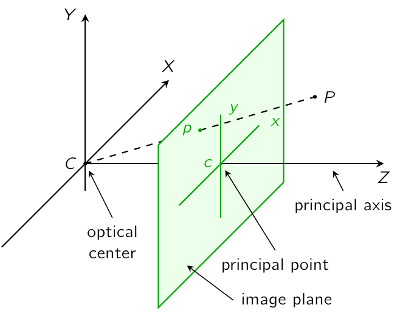
There are two coordinate-systems: The camera coordinate system  and the image coordinate system
  . Note that the coordinates of
  and
and  are arbitrary but fixed, so don’t mix them up with the coordinate systems.
We look at the scene above from the side:
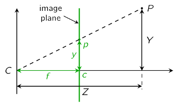
 is the distance between the optical center and the image plane and called the focal length. Due to the intercept theorem we get the following equations:
![\[ \frac{y}{f} = \frac{Y}{Z} \quad\Leftrightarrow\quad y = \frac{fY}{Z} \qquad\text{and}\qquad \frac{x}{f} = \frac{X}{Z} \quad\Leftrightarrow\quad x = \frac{fX}{Z} \]](form_31.png)
The can combine these two equation to a vector:

We now take a quick look at the most important characteristics of homogeneous coordinates. If you’ve never heard of homogeneous coordinates, you should catch up this topic.
Map a point to its homogeneous coordinates:

Equivalence of homogeneous coordinates:

given in homogeneous coordinates  :
:

You should keep these relations in mind.
We now map our points to their homogeneous coordinates as in (2):
![\[ P = \begin{pmatrix} X \\ Y \\ Z \end{pmatrix} \mapsto \begin{pmatrix} X \\ Y \\ Z \\ 1 \end{pmatrix} = \tilde{P},\quad p = \begin{pmatrix} x \\ y \end{pmatrix} \mapsto \begin{pmatrix} x \\ y \\ 1 \end{pmatrix} = \tilde{p}. \]](form_37.png)
This leads us to our equation (1) in homogeneous coordinates
![\[ \begin{pmatrix} x \\ y \end{pmatrix} = \begin{pmatrix} fX/Z \\ fY/Z \end{pmatrix} \quad\Rightarrow\quad \begin{pmatrix} x \\ y \\ 1 \end{pmatrix} = s \begin{pmatrix} fX/Z \\ fY/Z \\ 1 \end{pmatrix} \stackrel{\text{(3)}}{=} s \begin{pmatrix} fX \\ fY \\ Z \end{pmatrix}, \]](form_38.png)
where  represents the factor
  of (3). We can write this equation in the following way:
![\[ \begin{pmatrix} x \\ y \\ 1 \end{pmatrix} = s \begin{pmatrix} f & 0 & 0 & 0 \\ 0 & f & 0 & 0 \\ 0 & 0 & 1 & 0 \end{pmatrix} \begin{pmatrix} X \\ Y \\ Z \\ 1 \end{pmatrix} \]](form_41.png)
We assumed that the origin of the image coordinate system is located in the images’s center, so far. But often that is not the case. Therefore, we add an offset to the image point:
![\[ \begin{pmatrix} x \\ y \\ 1 \end{pmatrix} = s \begin{pmatrix} fX/Z + \hat{c}_x \\ fY/Z + \hat{c}_y \\ 1 \end{pmatrix} = s \begin{pmatrix} fX + \hat{c}_xZ \\ fY + \hat{c}_yZ \\ Z \end{pmatrix} = s \begin{pmatrix} f & 0 & \hat{c}_x & 0 \\ 0 & f & \hat{c}_y & 0 \\ 0 & 0 & 1 & 0 \end{pmatrix} \begin{pmatrix} X \\ Y \\ Z \\ 1 \end{pmatrix}. \]](form_42.png)
Until now we used  and
and  in units of length, which is not appropriate to pixel-related digital images. Hence, we introduce
  and
and  , which are the number of pixels per unit of length ([pixel/length]) in
  - and
- and  -direction. We then get pixels as unit:

This leads to

with the camera matrix
![\[ \mathbf{C} = \begin{pmatrix} f_x & 0 & c_x \\ 0 & f_y & c_y \\ 0 & 0 & 1 \end{pmatrix}. \]](form_51.png)
As a last step, we have to consider the different position and orientation of the depth- and RGB-camera. To combine the two resulting coordinate systems, we use a transformation which includes a rotation and a transformation. This can be written as the following matrix:
![\[ \mathbf{T} = \begin{pmatrix} r_{11} & r_{12} & r_{13} & t_1 \\ r_{21} & r_{22} & r_{23} & t_2 \\ r_{31} & r_{32} & r_{33} & t_3 \end{pmatrix} \]](form_52.png)
We can now extend our equation (5) to:

The fundamental formula

describes the relation between a threedimensional point in space captured by a camera and its equivalent, twodimensional point at the image plane.
The parameters are called:
 : intrisic parameters or intrinsics
  : extrinsic parameters or extrinsics
It is important to understand, that our model (excepted the transformation) has been derived for one general camera. In context of Kinect you have seperate intrinsics for the depth- and RGB-camera!
In addation, we used the transformation to combine the coordinate systems of the depth- and RGB-camera. That implicates, that we only have got one transformation-matrix.
The application of our model/formula in context of Kinect is explained at class-description.
 Generated on Sat Jan 28 2012 13:51:49 for Kiretu by version 1.7.3 of


