|
 |
 |
 |
|
|


Advanced Software Practical
|
| |
|
Abstract
On the way to get rid of the unnecessary vegetation in the 3D scans, we developed three different algorithms, called Chainsaw Algorithm and 2D/3D Fretsaw Algorithm. Each algorithm has its pros and cons. The Chainsaw-Algorithm is very fast, but less accurate than the other two.
If only the bare ground is of interest, the given solution is the 2D Fretsaw Algorithm algorithm.
The 3D-Fretsaw Algorithm is more elegant, it's far more accurate than the Chainsaw and keeps more details than the 2D version. On the downside the calculation time is significantly higher.
3D Laser Scanners
A 3D laser scanner is a device that analyses a real-world object or environment to collect data on its shape and possibly its appearance (i.e. color). Many different technologies can be used to gain 3D-images of objects, each coming with its own limitations, advantages and costs. There are still limitations in the kind of objects that can be digitized by optical laser scanning technologies, as the scanning process encounters difficulties with shiny, mirroring or transparent objects.
Basic Functionality
An extremely short laser pulse is emitted by the scanner, hits an obstacle by which it is reflected and is then received again by the scanner. The measured time of flight is proportional to the distance between scanner and object. The applied laser type allows measurements independent from ambient light.
Applications:
- surveying (landscape, buildings, etc.)
- preservation of monuments, historic buildings and artifacts
- architecture (construction / reconstruction)
- scanning of objects and persons for 3D-movies and PC-games
- forensic securing
Scanner
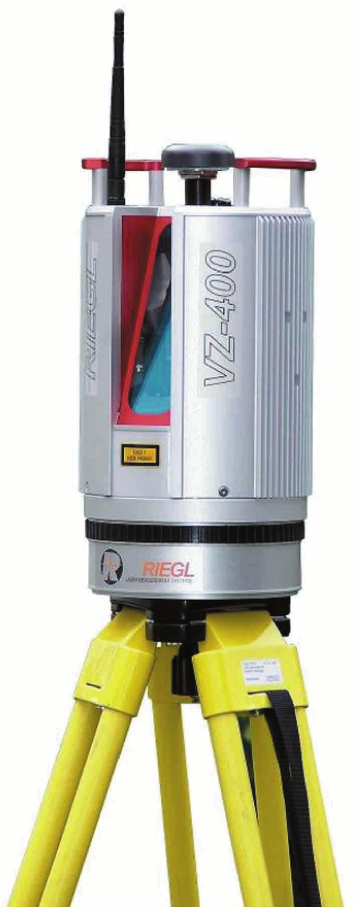
We worked with data from the Riegl VZ-400 Laser Scanner in our practical.
 Specifications:
- very fast Data acquisition
- integrated GPS-Receiver
- LAN,WLAN, USB2
- maximum range 600 m
- precision 5 mm
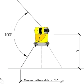
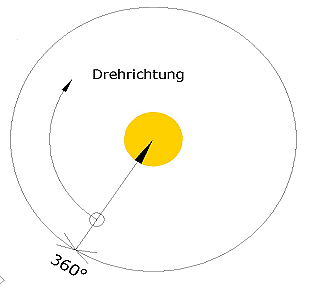
- scanrange horizontal 360°/ vertical 100° ( +60° / -40° )
The First Step
The first step in the development was to find a way of handling the huge amount of data. One single vertex in 3D space needs at least three floating point numbers for the position and another three for the color information. Our given 3D scans include up to 16 million vertices, so even actual computers could reach their limits pretty fast.
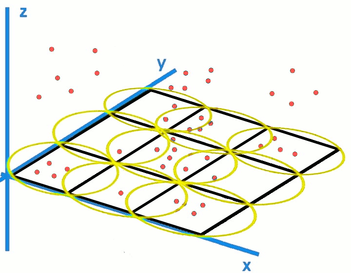
We have chosen to separate the data into 2D cells. It can be imagined as a 2D grid overlaying the 3D scan. So it's possible to decide locally inside a cell which points will be kept or deleted.
Naturally, the cell size determines the accuracy of the results. A finer grid allows a very good approximation of the underlying surface, but is also unresistant against outliers and requires more calculation time. All three algorithms provide the possibility for the user to change the grid size to achieve the best outcome.
The question remaining is, how to decide quickly which vertices are in the current cell. The answer is given in the next paragraph.
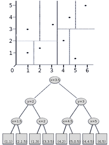
KD-Tree
The KD-tree is a data structure developed to find nearest neighbors within a given range in k-dimensional space very quickly.
Basically, the search domain will be iteratively separated to get a hierarchical tree structure.
The following search operation only needs an average time of O(log(n)) to find the closest points.
The Chainsaw and the 2D Fretsaw Algorithm work solely with a 2D-Tree, whereas the 3D Fretsaw Algorithm additionally needs the 3D variant.
|
|
 |
 |
 |
 |
|