|
 |
 |
 |
|
|


Advanced Software Practical
|
| |
|
Comparision of the Algorithms
Chainsaw Algorithm
- very fast
- works locally and provides good results even with slight uphill grades
- 2D Tree is needed
2D-Fretsaw Algorithm
- good performance
- moderate recognition of objects
- little additional costs (only 2D-Tree is needed)
3D-Fretsaw Algorithm
- computationally intensive
- improved recognition of objects
- 2D-Tree and 3D-Tree are needed
Performance Comparision
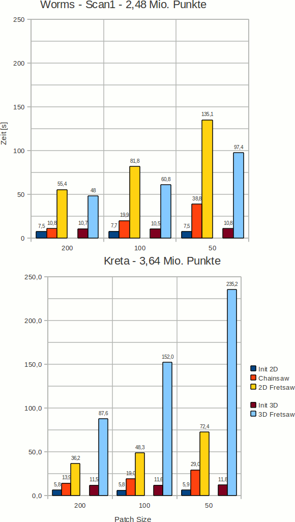
In the diagram above you see the results of performance measurements we did
on a laptop with a Pentium Core 2 Duo Processor (1.6 GHz).
We applied our three algorithms on two different data sets with three different patch (cell) sizes.
The times we called Init 2D and Init 3D give the time needed to build up the KD-trees (one tree for 2D and
two trees for 3D).
In the first scan, our 3D-Fretsaw-Algorithm clearly outperforms the 2D-variant. We guess here the data is sorted
in a better way, so that the 3D-algorithm doesn't need to switch between branches as frequently as in the 2D variant.
2D Fretsaw Algorithm
vs.
3D Fretsaw Algorithm
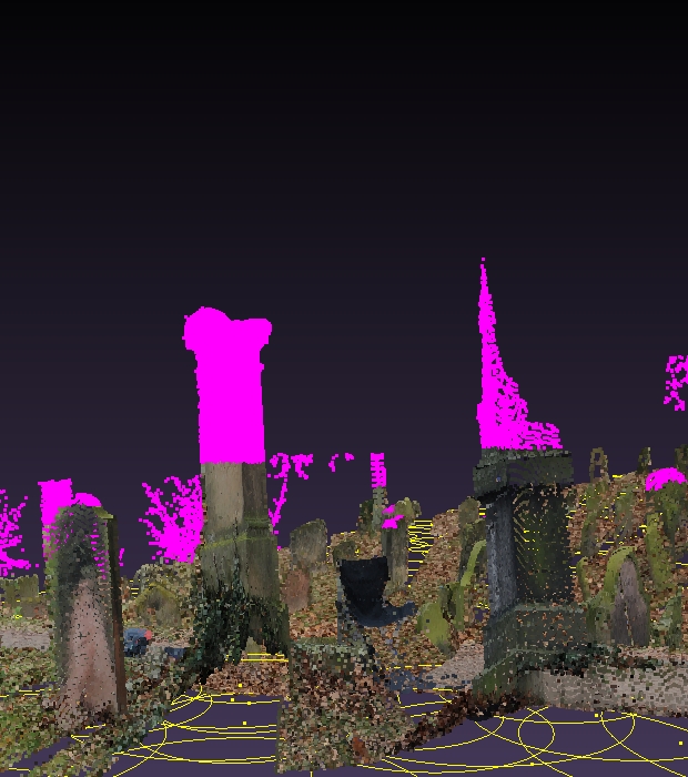
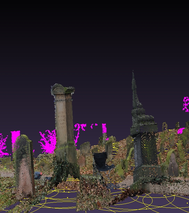
In the pictures above deleted points are marked in margenta. As you can see, important objects (gravestones) are preserved by the 3D Fretsaw Algorithm.
Results
Scan from Crete - Doline
In the following scan from Crete, you can clearly see the benefit of our algorithm in the basement of the doline, where the scanner was positioned.
Before Fretsaw-Algorithm
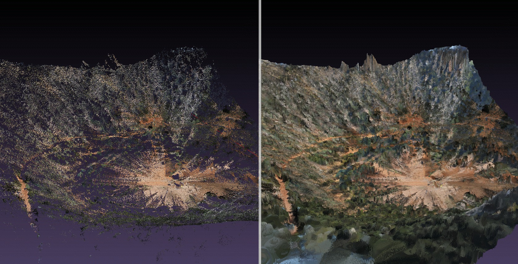
left: point cloud
right: generated mesh from point cloud
After Fretsaw-Algorithm
left: point cloud
right: generated mesh from point cloud
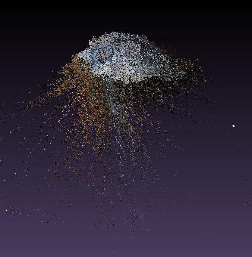
Old Castle
In the following, you see a terrain scan inside a thick forest, where only the surface is of interest.
In this case the 2D-Fretsaw Algorithm is the first choice to delete the foilage.
Unmodified Point Cloud
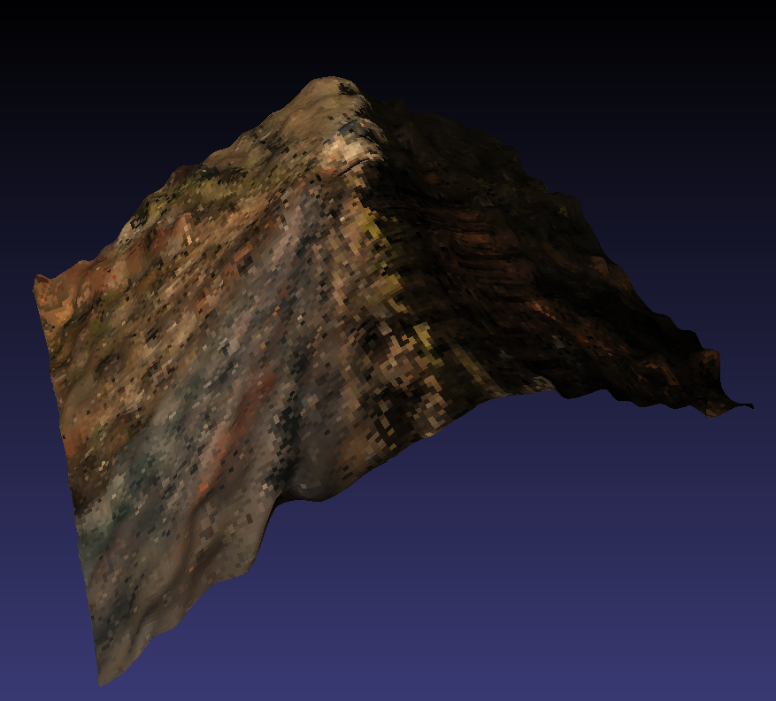
After 2D-Fretsaw Algorithm

Resulting Mesh (colored)
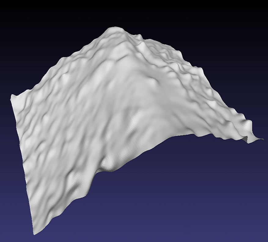
Resulting Mesh (non-colored with diffuse shading)
 |
|
 |
 |
 |
 |
|