Simplicial Complex
To represent topological spaces in computer, we need to discretize them. For this purpose, we use the simplicies. A simplex is a generalization of the notion of a triangle or tetrahedron to arbitrary dimensions. For example, a 0-simplex is a point, a 1-simplex is a line segment, a 2-simplex is a triangle, a 3-simplex is a tetrahedron
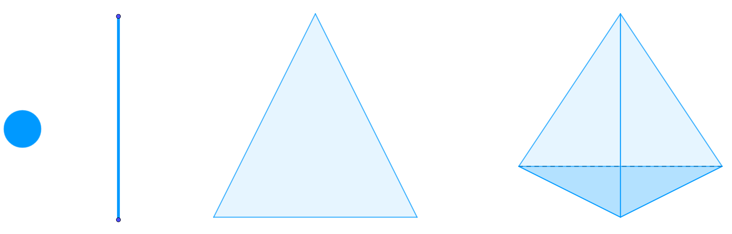
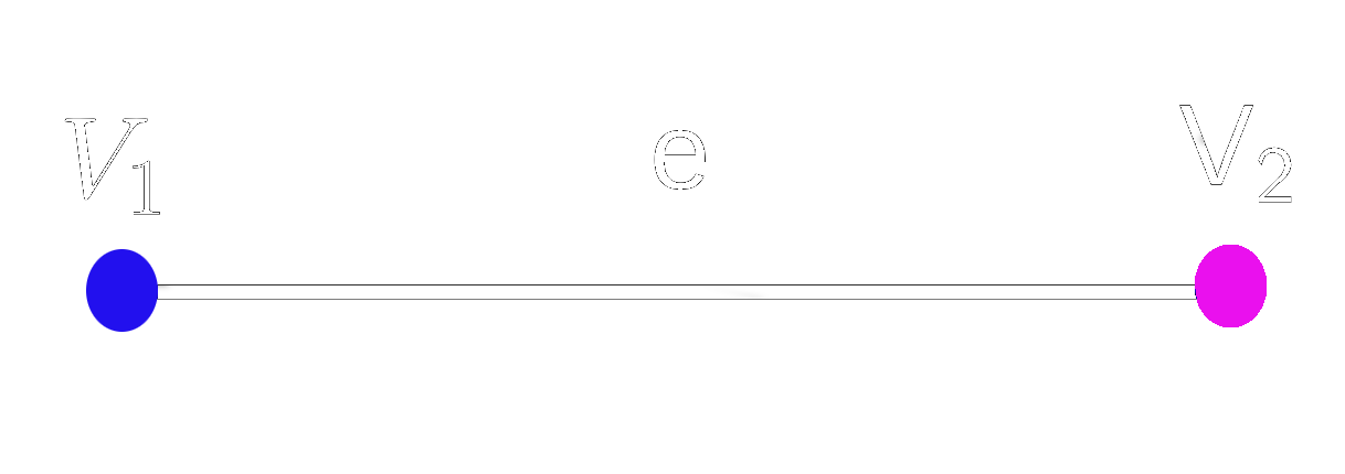
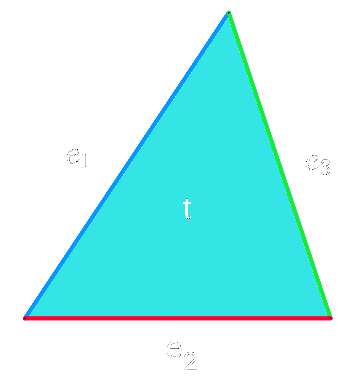
Every simplex with dimension > 0 has faces. A simplex β with dimension d has d+1 faces with dimension d-1. To understand this, we use the following concrete examples.
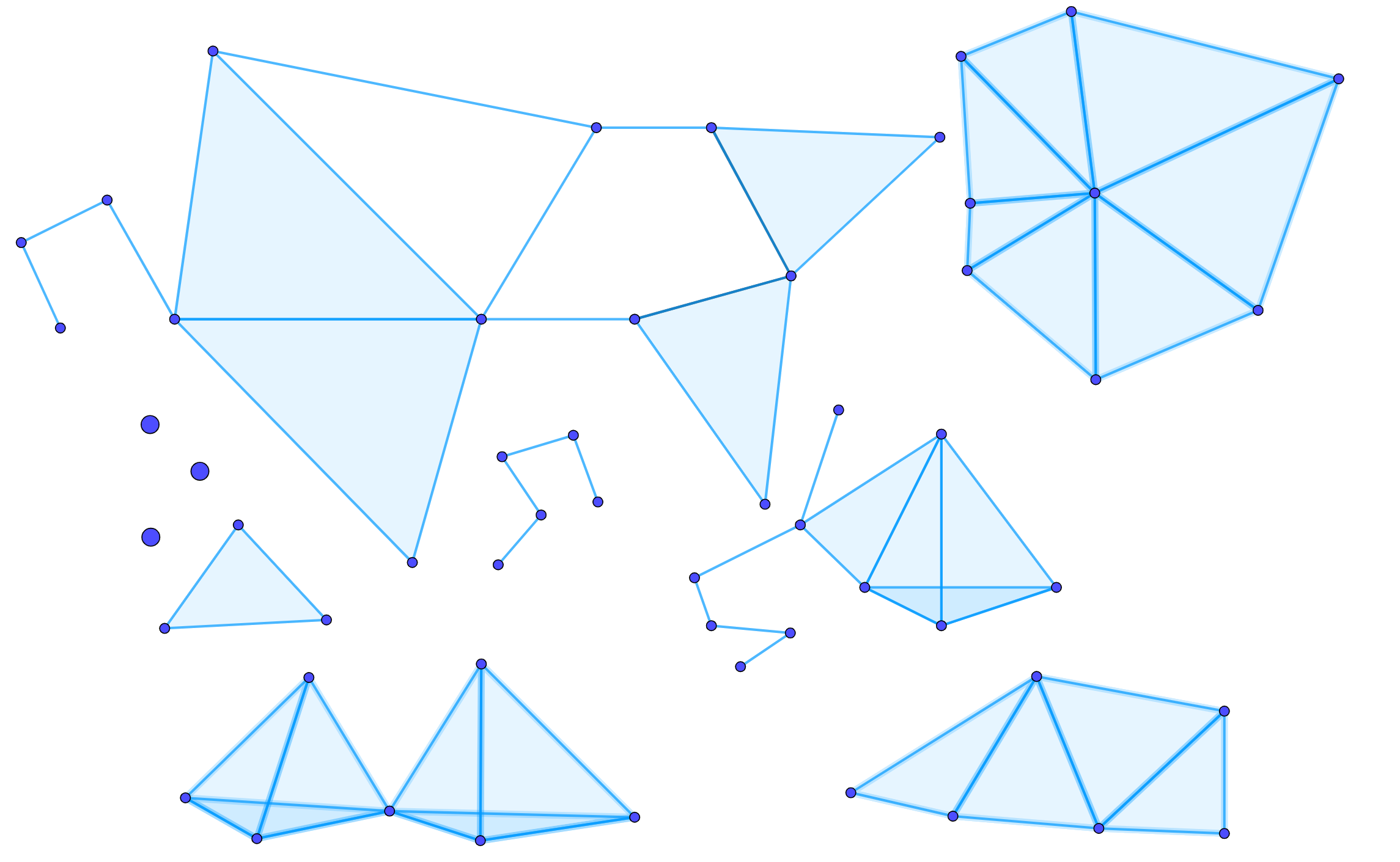
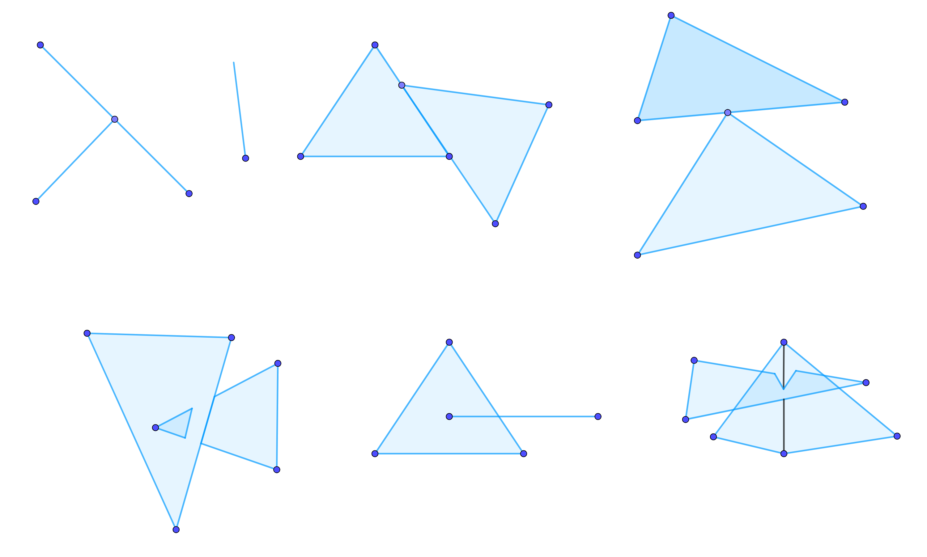
Now, we want to give the main definiton of this section. A simplicial complex $\mathcal{K}$ is a set of simplices that satisfies the following conditions:
- 1. Every face of a simplex from $\mathcal{K}$ is also in $\mathcal{K}$.
- 2.The non-empty intersection of any two simplices $\sigma_1,\sigma_2 \in \mathcal{K}$ is a face of both $\sigma_1$ and $\sigma_2$.
Triangulation
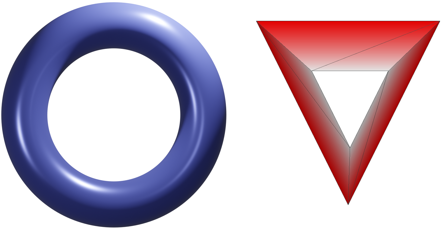
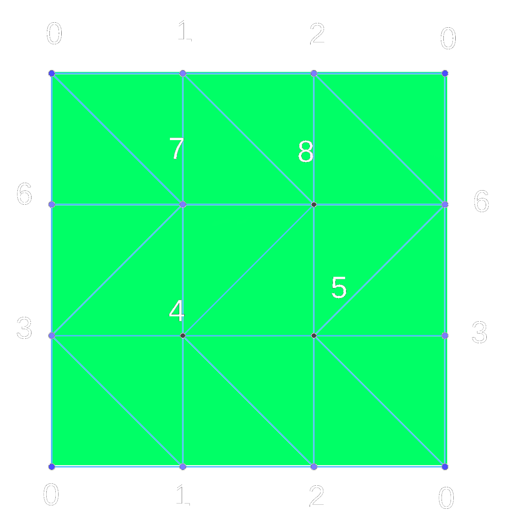
A triangulation of topological space X is a simplicial complex $\mathcal{K}$ with a homeomorphism $h: \mathcal{K}\rightarrow X$. If we take the torus as an example of a topological space, we can find many triangulation of it, but in the next image we see the triangulation of the topological spaces with small number of simplices.
Discrete Morse Function
Let $\mathcal{K}$ be a simplicial complex. A function $f:\mathcal{K}\rightarrow \mathbb{R}$ is a discrete Morse function if:
- 1. The number of $\{\beta^{(p+1)}>\alpha^p \mid f(\beta) \leq f(\alpha)\}\leq 1$
- 2. The number of $\{\gamma^{(p-1)}<\alpha^p \mid f(\gamma) \geq f(\alpha)\}\leq 1$
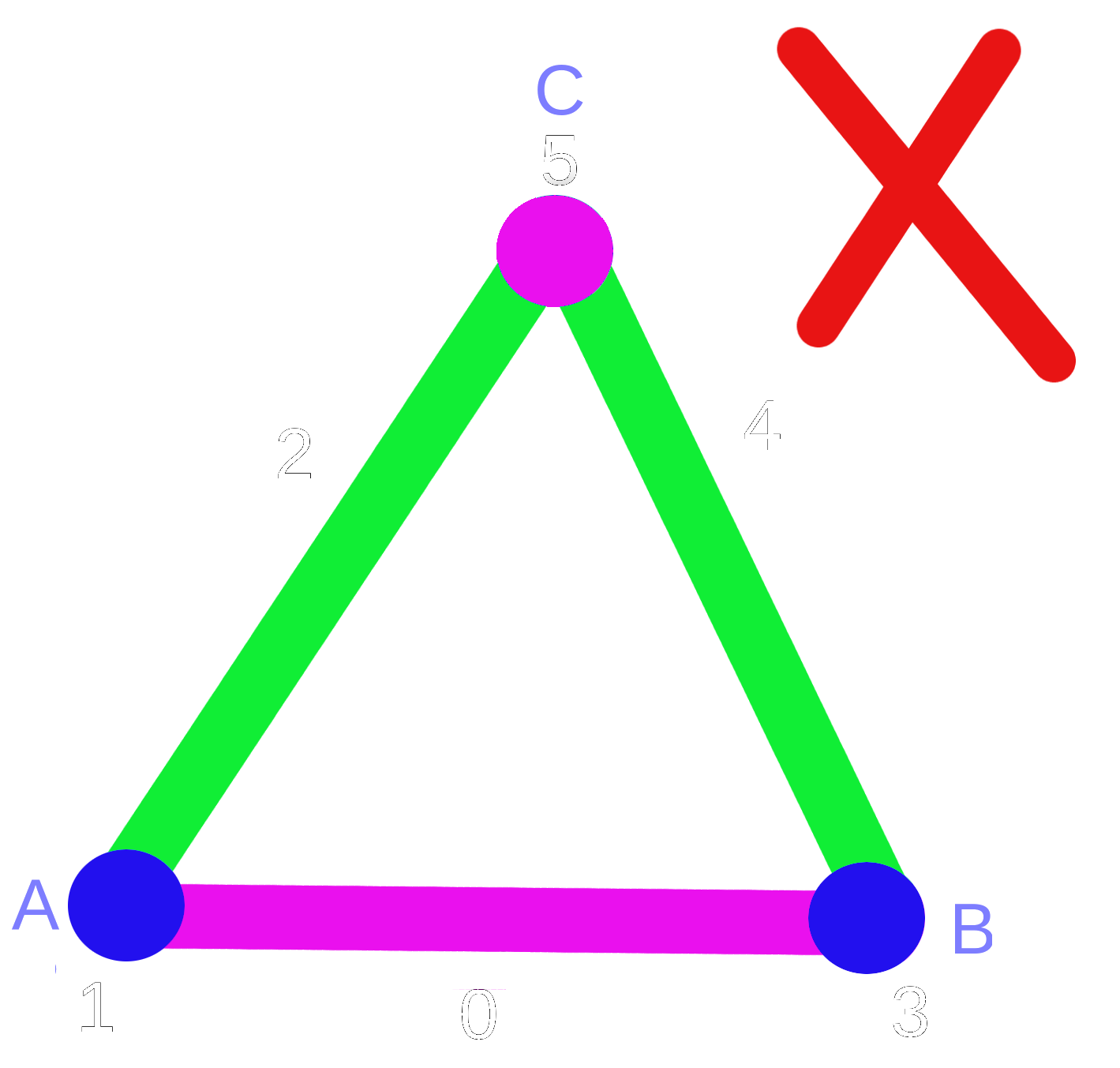
In the next example, the 1-d simplicial complex has discrete Morse function because the two conditions of the definiton are fulfilled.
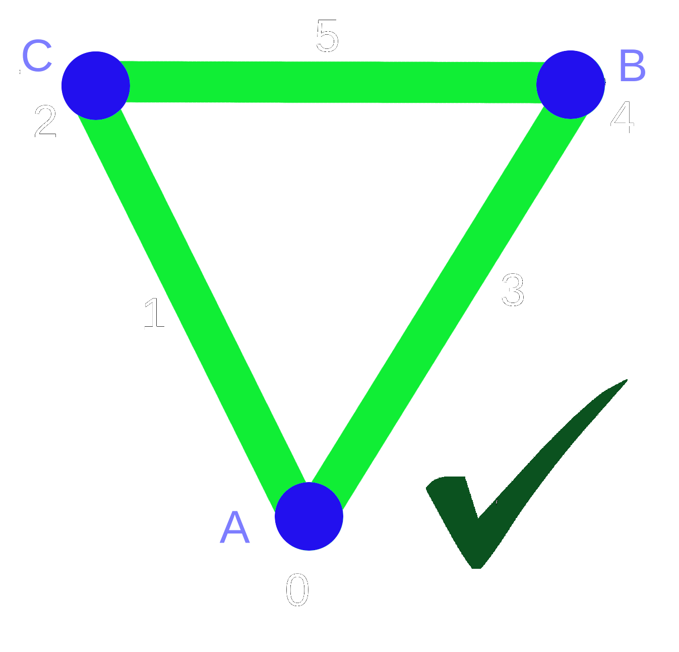
Let $\mathcal{K}$ be a simplicial complex and f is a discrete Morse function, we say that a simplex in $\mathcal{K}$ is critical if:
1.The number of $\{\beta^{(p+1)}>\alpha^p \mid f(\beta) \leq f(\alpha)\}=0$
2.The number of $\{\beta^{(p+1)}>\alpha^p \mid f(\beta) \leq f(\alpha)\}=0$
If we look at the discrete Morse function in the last figure we can recognize two critical cells . The first critical cell is the point A because A has no coface with smaller or equal function value and has no faces with greater function value. The second critical cell is the edge BC because all the faces of BC have less function value and BC has no cofaces.
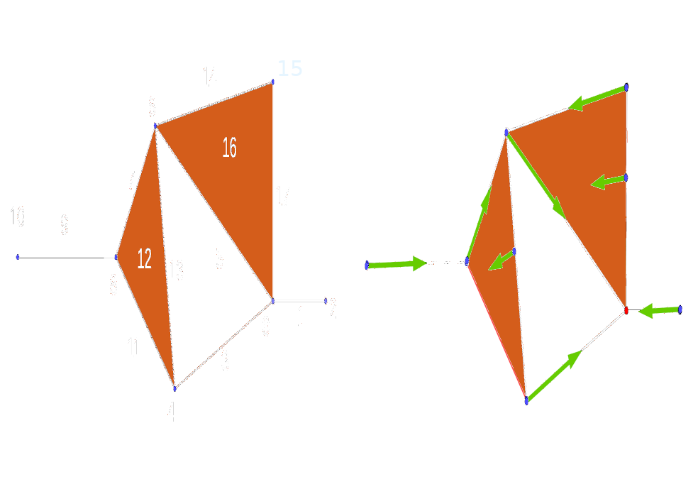
Gradient vector field
If we have a simplicial complex with discrete Morse function f, we know from the definiton that every simplex $\beta$ has at maximum one face $\alpha$ with $f(\alpha) \geq f(\beta)$. If we draw an arrow from $\alpha$ to $\beta$ (the tail on $\alpha$ and the head on $\beta$) this will lead us to the fact that every simplex $\alpha$ in the complex is one of the following:
1. $\alpha$ is the tail of exactly one arrow.
2. $\alpha$ is the head of exactly one arrow.
3. $\alpha$ is neither the tail nor the head of any arrow.
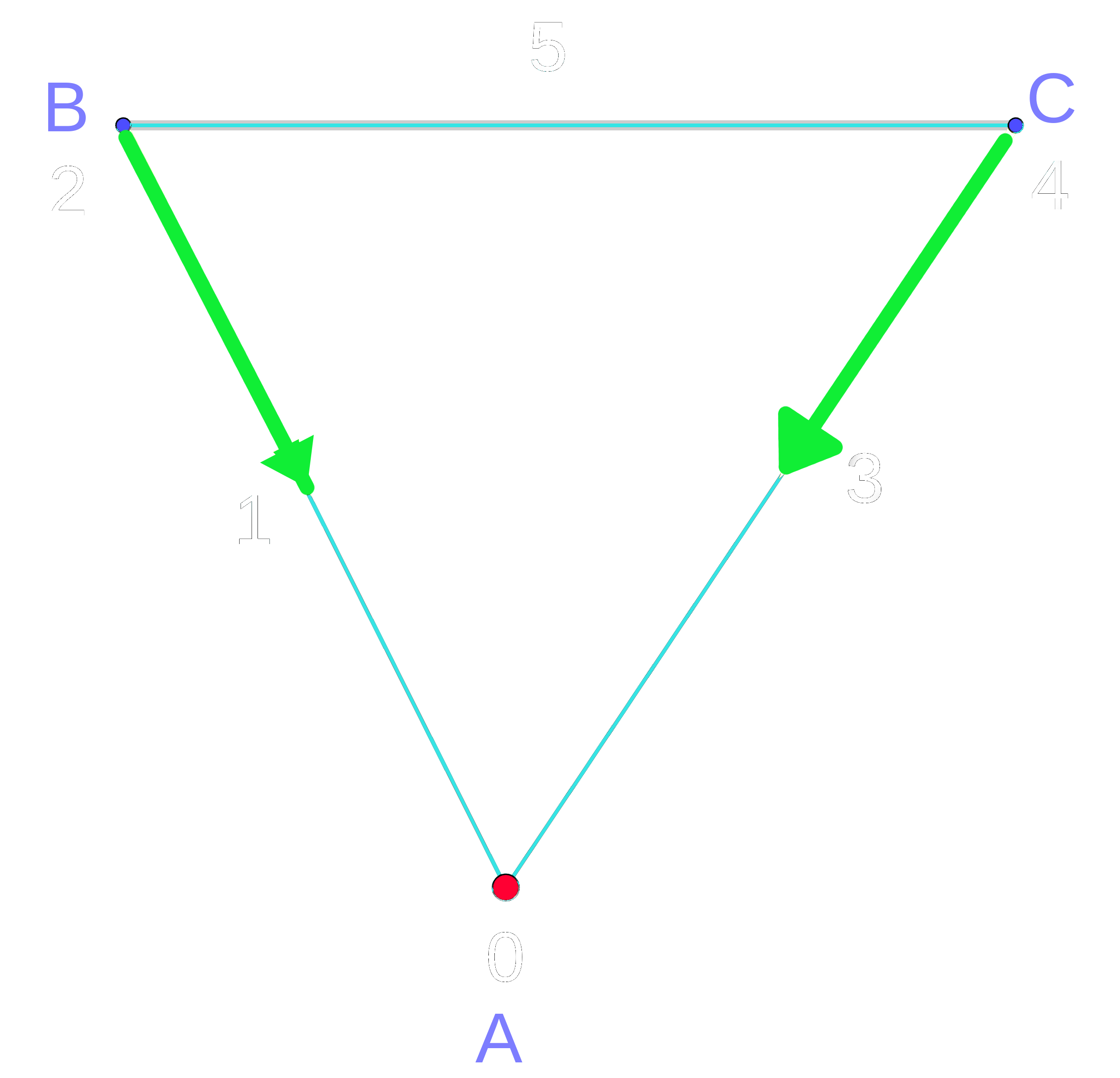
. It's more easy to work with those arrows than working with concrete discrete Morse function. In fact, this gradient vector field contains all of the information that we will need to know about the function for most applications. The next is another example of gradient vector field.